Unconfoundedness
We call 'Uncofoundedness' a scenario where a treatment is not randomly assigned to participants, so confounders effect on treatment assignment and outcome. We have client - level data. Confounders were measured before treatment and outcome after
Let's look at the example:
In our ecosystem we have a product, which effect on LTV we want to estimate
Treatment - first purchase in product.
Outcome - LTV after first purchase.
We will test hypothesis:
- There is no difference in LTV between treatment and control groups.
- There is a difference in LTV between treatment and control groups.
Causal Assumptions
Unconfoundedness: We control all confounders
Overlap: propensity distributions overlap
SUTVA: no interference and consistent treatment definitions. By design
DML works correctly: nuisance functions are correctly specified
No leakage: confounders are measured before treatment
Data
For the analysis you need data in pandas dataframe:
- treatment column in binary format (1/0)
- outcome column numeric format, measured after treatment time
- user_id column (Optional, but useful)
- confounders columns (Optional, measured before treatment time, numeric format, used for causal assumption check)
We will take data from Causalis DGP.. Read more at https://causalis.causalcraft.com/articles/generate_obs_hte_26_rich
| user_id | y | d | tenure_months | avg_sessions_week | spend_last_month | age_years | income_monthly | prior_purchases_12m | support_tickets_90d | premium_user | mobile_user | urban_resident | referred_user | m | m_obs | tau_link | g0 | g1 | cate | |
|---|---|---|---|---|---|---|---|---|---|---|---|---|---|---|---|---|---|---|---|---|
| 0 | 1 | 0.000000 | 0.0 | 28.814654 | 1.0 | 77.936767 | 50.234101 | 1926.698301 | 1.0 | 2.0 | 1.0 | 1.0 | 1.0 | 0.0 | 0.045453 | 0.045453 | 0.089095 | 8.137981 | 9.142395 | 1.004414 |
| 1 | 2 | 80.099611 | 1.0 | 25.913345 | 3.0 | 53.777740 | 28.115859 | 5104.271509 | 3.0 | 0.0 | 1.0 | 1.0 | 0.0 | 1.0 | 0.041514 | 0.041514 | 0.246679 | 60.459257 | 78.817307 | 18.358049 |
| 2 | 3 | 6.400482 | 1.0 | 24.969929 | 10.0 | 134.764322 | 22.907062 | 5267.938255 | 8.0 | 3.0 | 0.0 | 1.0 | 1.0 | 0.0 | 0.052593 | 0.052593 | 0.162968 | 7.712855 | 9.138577 | 1.425723 |
| 3 | 4 | 2.788238 | 0.0 | 40.655089 | 5.0 | 59.517074 | 31.970490 | 6597.327018 | 3.0 | 2.0 | 1.0 | 1.0 | 1.0 | 0.0 | 0.036221 | 0.036221 | 0.188755 | 25.386510 | 31.159932 | 5.773422 |
| 4 | 5 | 0.000000 | 0.0 | 18.560899 | 3.0 | 74.370930 | 39.237248 | 4930.009628 | 5.0 | 1.0 | 1.0 | 1.0 | 0.0 | 0.0 | 0.036343 | 0.036343 | 0.174757 | 15.359250 | 18.600227 | 3.240977 |
CausalData(df=(100000, 14), treatment='d', outcome='y', confounders=['tenure_months', 'avg_sessions_week', 'spend_last_month', 'age_years', 'income_monthly', 'prior_purchases_12m', 'support_tickets_90d', 'premium_user', 'mobile_user', 'urban_resident', 'referred_user'], user_id='user_id')
EDA
| treatment | count | mean | std | min | p10 | p25 | median | p75 | p90 | max | |
|---|---|---|---|---|---|---|---|---|---|---|---|
| 0 | 0 | 95051 | 76.087138 | 240.800713 | 0.0 | 0.0 | 0.0 | 8.39544 | 64.859278 | 190.227900 | 21396.007575 |
| 1 | 1 | 4949 | 58.506172 | 199.485625 | 0.0 | 0.0 | 0.0 | 0.00000 | 36.958280 | 148.837193 | 5143.642132 |
Our data has strong treatment class disbalance. Only 5% of sample activated in treatment.
Treatment group has lower mean LTV. It's too early to draw conclusions.
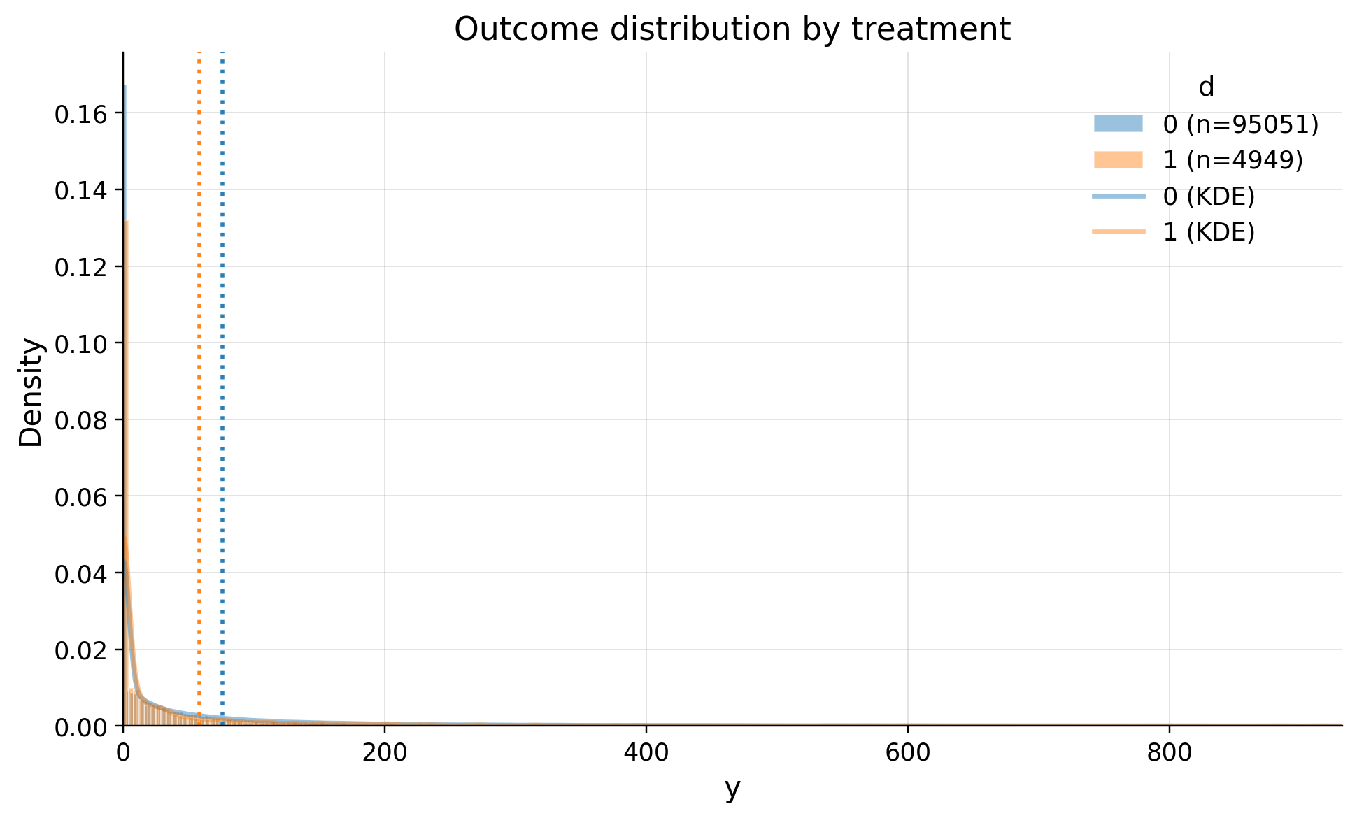
We see large right tale
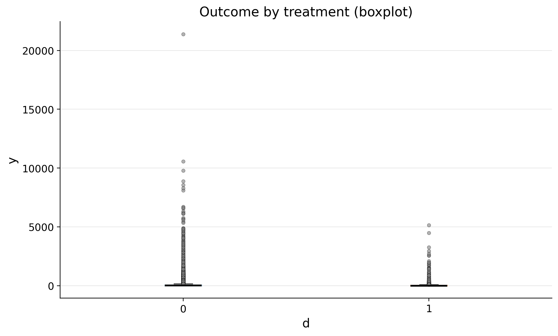
| treatment | n | outlier_count | outlier_rate | lower_bound | upper_bound | has_outliers | method | tail | |
|---|---|---|---|---|---|---|---|---|---|
| 0 | 0 | 95051 | 11300 | 0.118884 | -97.288916 | 162.148194 | True | iqr | both |
| 1 | 1 | 4949 | 721 | 0.145686 | -55.437420 | 92.395699 | True | iqr | both |
We see many outliers. It's common situation for LTV metric. Dropping them will lead to a biased conclusion
| confounders | mean_d_0 | mean_d_1 | abs_diff | smd | ks_pvalue | |
|---|---|---|---|---|---|---|
| 0 | premium_user | 0.751807 | 0.591837 | 0.159970 | -0.345721 | 0.00000 |
| 1 | income_monthly | 4549.385190 | 3918.058798 | 631.326392 | -0.277611 | 0.00000 |
| 2 | spend_last_month | 89.091801 | 67.375389 | 21.716412 | -0.268360 | 0.00000 |
| 3 | support_tickets_90d | 0.984545 | 1.259244 | 0.274699 | 0.253974 | 0.00000 |
| 4 | avg_sessions_week | 5.047753 | 4.230148 | 0.817606 | -0.201735 | 0.00000 |
| 5 | prior_purchases_12m | 3.904220 | 3.513639 | 0.390581 | -0.189372 | 0.00000 |
| 6 | tenure_months | 28.740100 | 25.559161 | 3.180939 | -0.184156 | 0.00000 |
| 7 | age_years | 36.435984 | 34.809083 | 1.626901 | -0.144142 | 0.00000 |
| 8 | referred_user | 0.271486 | 0.307133 | 0.035647 | 0.078671 | 0.00001 |
| 9 | urban_resident | 0.600793 | 0.568802 | 0.031991 | -0.064954 | 0.00013 |
| 10 | mobile_user | 0.874573 | 0.870075 | 0.004498 | -0.013477 | 0.99998 |
As we see clients are differ on this confounders. We need to controll them to make causal inference
Inference
ATTE is right estimand here. We will estimate effect on clients that were treated, had first purchase in our product
Read more about DML at https://causalis.causalcraft.com/articles/unconfoundedness-model
| value | |
|---|---|
| field | |
| outcome | y |
| estimand | ATTE |
| model | IRM |
| value | 9.9026 (ci_abs: 4.4731, 15.3320) |
| value_relative | 20.3741 (ci_rel: 8.3518, 32.3964) |
| alpha | 0.0500 |
| p_value | 0.0004 |
| is_significant | True |
| n_treated | 4949 |
| n_control | 95051 |
| treatment_mean | 58.5062 |
| control_mean | 76.0871 |
| time | 2026-08-27 |
Our estimate is 12.1542 dollars (ci_abs: 7.7933, 16.5152). Mean in treatment group is 58.5062 dollars, so without our product it would be 46.3520 dollars.
Refutation
Unconfoundedness
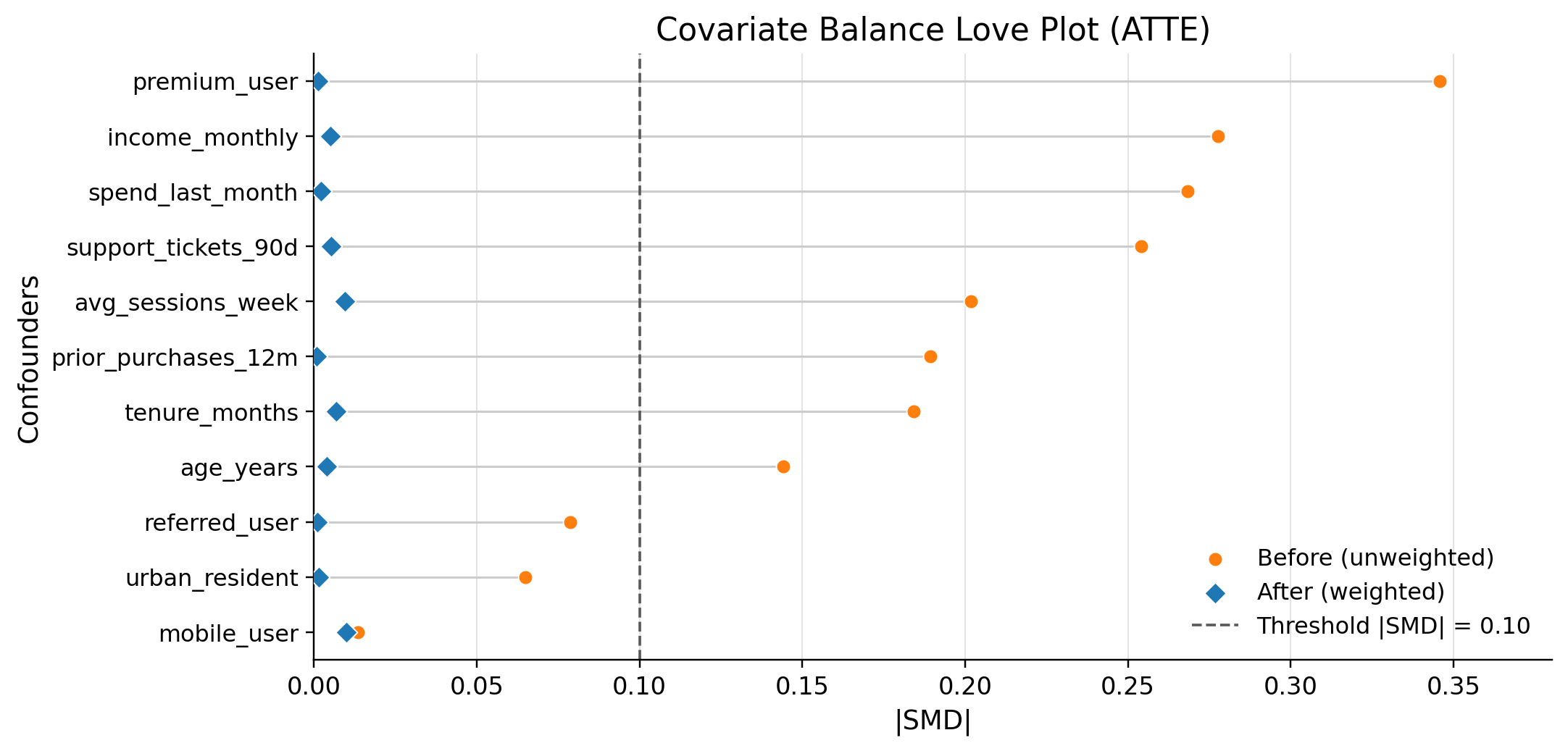
balance_max_smd is 0.011635 so dml specification dealt with controlling confounders
Sensitivity
By default, rank_confounder_clusters(...).head(3) selects two clusters by importance_d * importance_y, then the cluster with the highest importance_d among those not already selected. This reuses existing importances without extra model fits. Scores are unchanged, but mixed ordering is not necessarily descending by score. Use ranking_method="joint" to restore the previous ordering. This is a screening heuristic and does not guarantee higher benchmark r2_d.
| cluster_id | features | n_features | importance_d | importance_g0 | importance_g1 | importance_y | score | |
|---|---|---|---|---|---|---|---|---|
| 0 | 1 | [avg_sessions_week] | 1 | 0.092340 | 0.279259 | 0.200673 | 0.239966 | 0.022158 |
| 1 | 0 | [tenure_months] | 1 | 0.164019 | 0.116581 | 0.106571 | 0.111576 | 0.018301 |
| 2 | 2 | [spend_last_month] | 1 | 0.175976 | 0.068335 | 0.075962 | 0.072149 | 0.012696 |
PASS PASS: the practically meaningful effect is robust to hidden confounding comparable to every primary benchmark. Every primary bias-aware confidence interval satisfies the positive decision rule (ci_lower > 0). The reported stress-test margin is limited. DoubleML boundary calibration was used for ['rank_2_cluster_0', 'rank_3_cluster_2'].
SUTVA
1.) Are your clients independent (i). Outcome of ones do not depend on others? 2.) Are all clients have full window to measure metrics? 3.) Do you measure confounders before treatment and outcome after? 4.) Do you have a consistent label of treatment, such as if a person does not receive a treatment, he has a label 0?
SUTVA is untestable from data alone, so we call it true by design
Score
| metric | value | flag | |
|---|---|---|---|
| 0 | psi_p99_over_med | 63.832306 | RED |
| 1 | psi_kurtosis | 12446.186007 | RED |
| 2 | max_|t|_g0 | 0.669255 | GREEN |
| 3 | max_|t|_m | 1.781017 | GREEN |
| 4 | oos_max_abs_t | 0.000015 | GREEN |
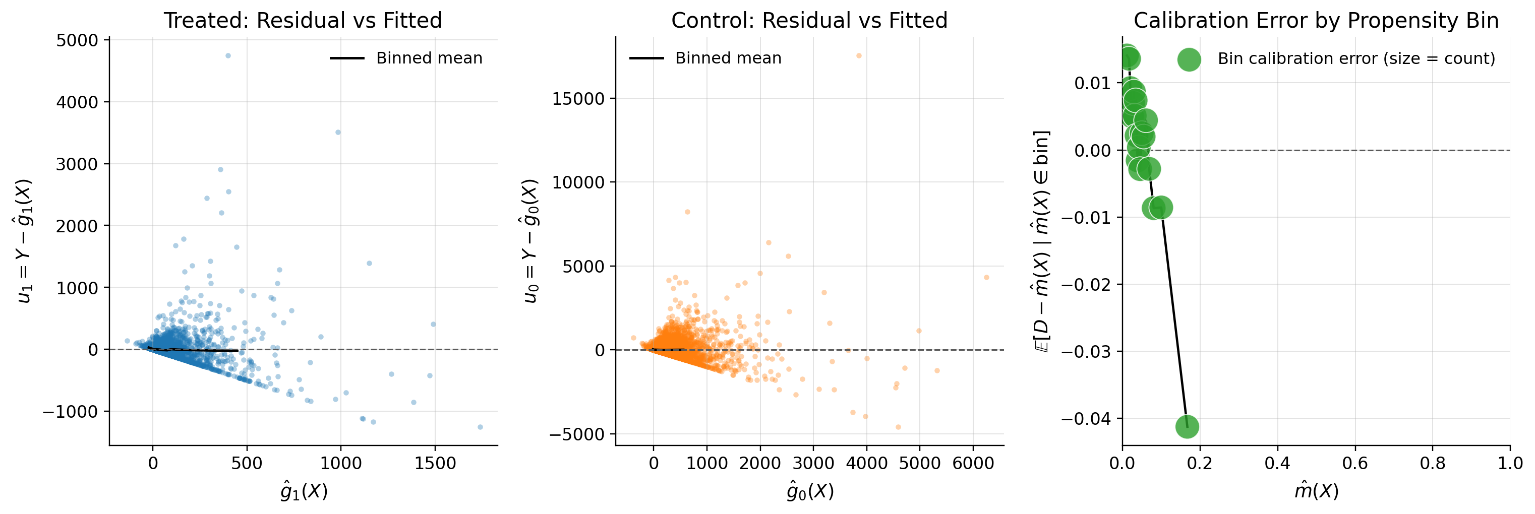
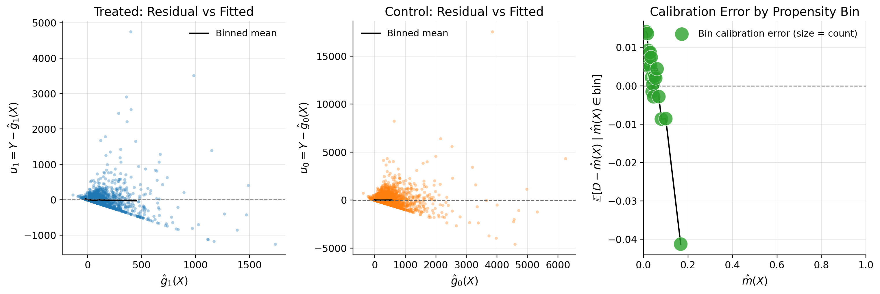
DML is specified correctly. There are many outliers in data that effect the score
Overlap
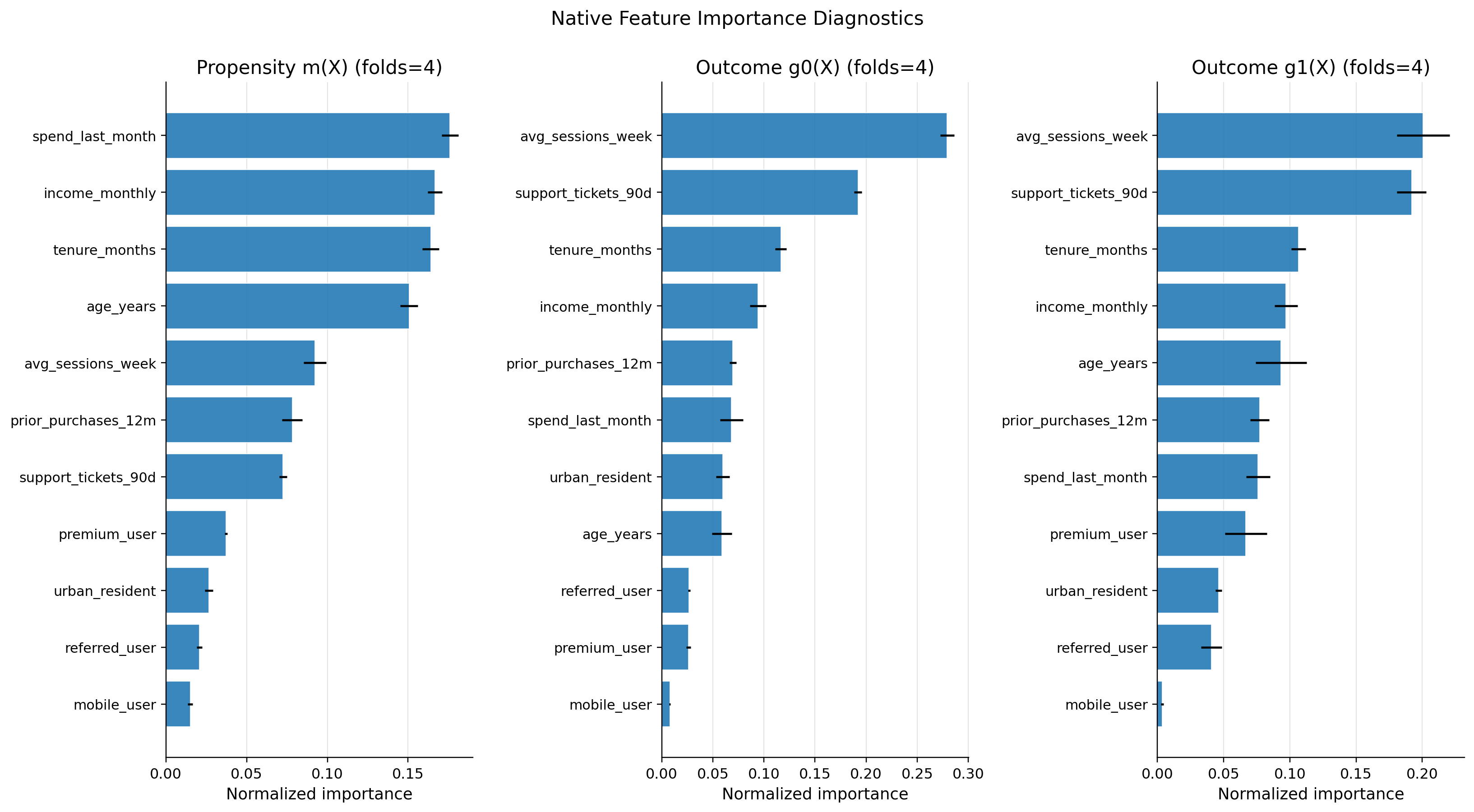
Customers are not inclined to activate the our product
| metric | value | flag | |
|---|---|---|---|
| 0 | edge_0.01_below | 0.018790 | GREEN |
| 1 | edge_0.01_above | 0.000000 | GREEN |
| 4 | KS | 0.196517 | GREEN |
| 6 | support_rate | 0.999798 | GREEN |
| 7 | ESS_treated_ratio | 0.465148 | GREEN |
| 8 | ESS_control_ratio | 0.996909 | GREEN |
| 11 | ATT_identity_relerr | 0.005642 | GREEN |
| 13 | calib_ECE | 0.005459 | GREEN |
if calib_ECE is YELLOW/RED look at plot_propensity_reliability(dml_result)
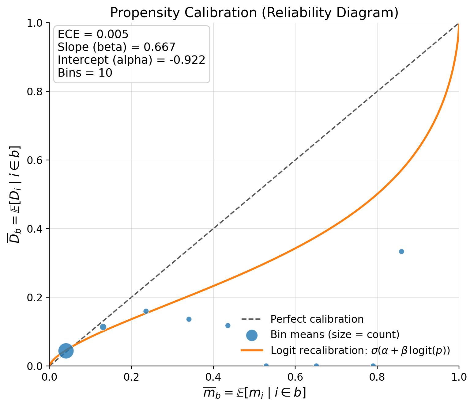
Logistic recalibration trend is a fitted correction curve for your predicted propensities.
The plot takes your original propensity p and fits this model:
corrected_p = sigmoid(alpha + beta * logit(p)) So the orange line answers:
If I recalibrate these predicted probabilities to better match observed treatment frequencies, what corrected probability would I use?
How to read it:
- If orange line matches the diagonal: predictions are already well calibrated
- If orange line is below the diagonal: model tends to overpredict treatment
- If orange line is above the diagonal: model tends to underpredict treatment
Rule of thumb:
- ECE near 0 and slope near 1: great
- ECE near 0 but slope far from 1: average calibration is fine, but probabilities are distorted in shape
- Many tiny bad bins + one huge good bin: visually noisy, but often not a major practical issue
Let's compare with oracle effect
Ground truth ATE is 19.40958652966079 Ground truth ATTE is 10.914991423363862
Conclusion
Estimated ATTE is 9.9026 (ci_abs: 4.4731, 15.3320) dollars. The DoubleML-compatible sensitivity protocol returns PASS for all three primary benchmarks, but with a limited robustness margin: tenure_months and income_monthly use boundary calibration (cf_d_raw < 0 clipped to cf_d=0, rho=1 fallback), while the rho=1 adversarial scenario for avg_sessions_week fails.