generate_obs_hte_26_rich()
This notebook presents the generate obs hte 26 rich research workflow and key analysis steps.
The generate_obs_hte_26_rich() function provides a more complex and realistic observational dataset. It features 11 confounders, complex dependencies (including derived features), a low treatment rate, and a Tweedie (zero-inflated Gamma) outcome model.
1. Confounders ()
The dataset contains 11 confounders :
- :
tenure_months - :
avg_sessions_week - :
spend_last_month - :
age_years - :
income_monthly - :
prior_purchases_12m - :
support_tickets_90d - :
premium_user - :
mobile_user - :
urban_resident - :
referred_user
Base Features Sampling: The base features are sampled using a Gaussian Copula with the following correlation matrix:
Derived Features: The remaining features are derived to mimic real-world behavioral dependencies:
- Premium User ():
- Mobile User ():
- Referred User ():
- Prior Purchases ():
- Support Tickets ():
2. Treatment Assignment ()
The treatment is assigned with a target rate of 5%: where with and
This design induces adverse selection (treated units can have lower observed outcomes than controls even when treatment helps on average).
3. Heterogeneous Treatment Effect ()
The treatment effect on the link (log-mean) scale is: and is clipped to .
Important: this clipping is for on the link scale, not for CATE itself.
4. Outcome Model ()
The outcome follows a Tweedie (Two-part Hurdle) model:
-
Zero-Inflation (Participation): with probability where , and the nonlinear components are:
-
Positive Outcome (Magnitude): If , then where . The baseline nonlinear part is: The oracle natural-scale CATE is always computed as where under the two-part model.
| y | d | tenure_months | avg_sessions_week | spend_last_month | age_years | income_monthly | prior_purchases_12m | support_tickets_90d | premium_user | mobile_user | urban_resident | referred_user | m | m_obs | tau_link | g0 | g1 | cate | |
|---|---|---|---|---|---|---|---|---|---|---|---|---|---|---|---|---|---|---|---|
| 0 | 0.000000 | 0.0 | 28.814654 | 1.0 | 77.936767 | 50.234101 | 1926.698301 | 1.0 | 2.0 | 1.0 | 1.0 | 1.0 | 0.0 | 0.045453 | 0.045453 | 0.089095 | 8.137981 | 9.142395 | 1.004414 |
| 1 | 80.099611 | 1.0 | 25.913345 | 3.0 | 53.777740 | 28.115859 | 5104.271509 | 3.0 | 0.0 | 1.0 | 1.0 | 0.0 | 1.0 | 0.041514 | 0.041514 | 0.246679 | 60.459257 | 78.817307 | 18.358049 |
| 2 | 6.400482 | 1.0 | 24.969929 | 10.0 | 134.764322 | 22.907062 | 5267.938255 | 8.0 | 3.0 | 0.0 | 1.0 | 1.0 | 0.0 | 0.052593 | 0.052593 | 0.162968 | 7.712855 | 9.138577 | 1.425723 |
| 3 | 2.788238 | 0.0 | 40.655089 | 5.0 | 59.517074 | 31.970490 | 6597.327018 | 3.0 | 2.0 | 1.0 | 1.0 | 1.0 | 0.0 | 0.036221 | 0.036221 | 0.188755 | 25.386510 | 31.159932 | 5.773422 |
| 4 | 0.000000 | 0.0 | 18.560899 | 3.0 | 74.370930 | 39.237248 | 4930.009628 | 5.0 | 1.0 | 1.0 | 1.0 | 0.0 | 0.0 | 0.036343 | 0.036343 | 0.174757 | 15.359250 | 18.600227 | 3.240977 |
Ground truth ATE is 19.409586529660793 Ground truth ATTE is 10.914991423363865
CausalData(df=(100000, 13), treatment='d', outcome='y', confounders=['tenure_months', 'avg_sessions_week', 'spend_last_month', 'age_years', 'income_monthly', 'prior_purchases_12m', 'support_tickets_90d', 'premium_user', 'mobile_user', 'urban_resident', 'referred_user'])
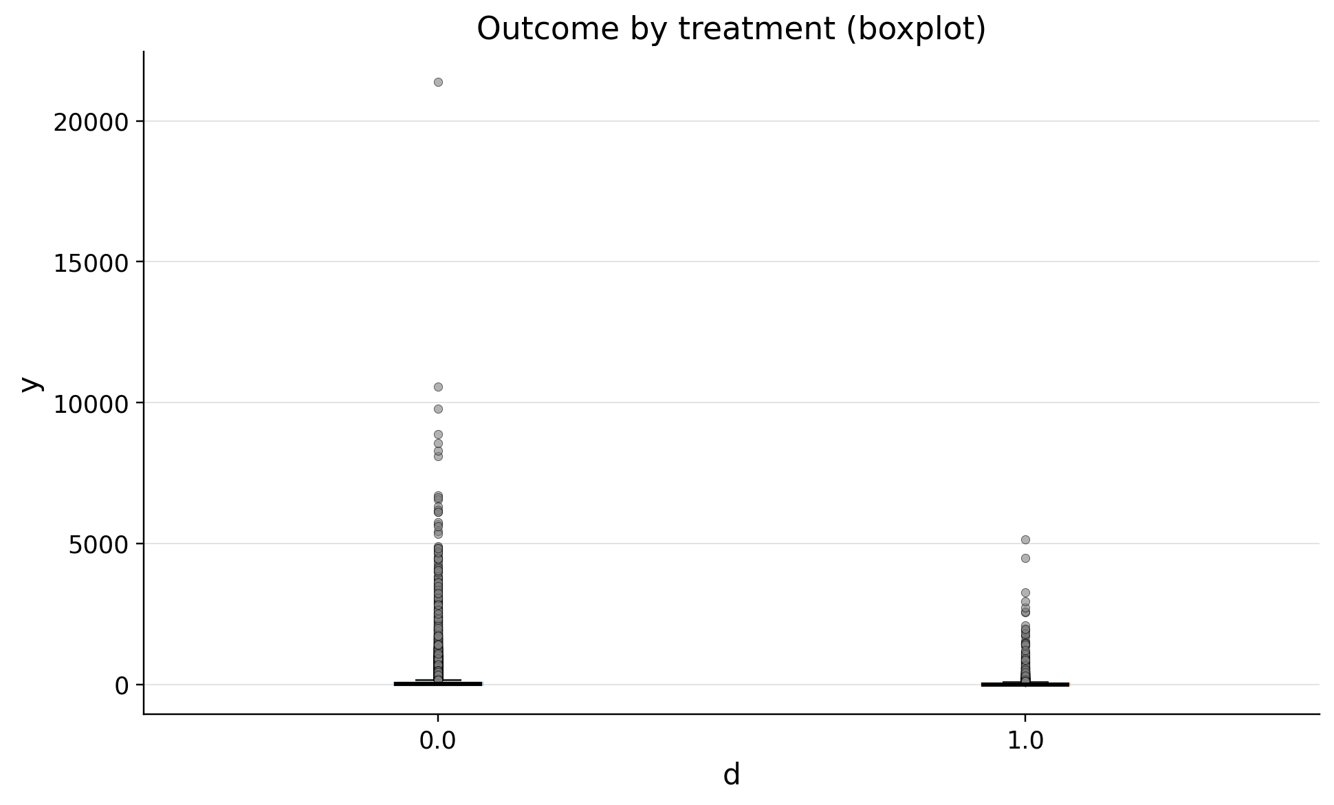
| treatment | count | mean | std | min | p10 | p25 | median | p75 | p90 | max | |
|---|---|---|---|---|---|---|---|---|---|---|---|
| 0 | 0.0 | 95051 | 76.087138 | 240.800713 | 0.0 | 0.0 | 0.0 | 8.39544 | 64.859278 | 190.227900 | 21396.007575 |
| 1 | 1.0 | 4949 | 58.506172 | 199.485625 | 0.0 | 0.0 | 0.0 | 0.00000 | 36.958280 | 148.837193 | 5143.642132 |

| treatment | n | outlier_count | outlier_rate | lower_bound | upper_bound | has_outliers | method | tail | |
|---|---|---|---|---|---|---|---|---|---|
| 0 | 0.0 | 95051 | 11300 | 0.118884 | -97.288916 | 162.148194 | True | iqr | both |
| 1 | 1.0 | 4949 | 721 | 0.145686 | -55.437420 | 92.395699 | True | iqr | both |
| confounders | mean_d_0 | mean_d_1 | abs_diff | smd | ks_pvalue | |
|---|---|---|---|---|---|---|
| 0 | premium_user | 0.751807 | 0.591837 | 0.159970 | -0.345721 | 0.00000 |
| 1 | income_monthly | 4549.385190 | 3918.058798 | 631.326392 | -0.277611 | 0.00000 |
| 2 | spend_last_month | 89.091801 | 67.375389 | 21.716412 | -0.268360 | 0.00000 |
| 3 | support_tickets_90d | 0.984545 | 1.259244 | 0.274699 | 0.253974 | 0.00000 |
| 4 | avg_sessions_week | 5.047753 | 4.230148 | 0.817606 | -0.201735 | 0.00000 |
| 5 | prior_purchases_12m | 3.904220 | 3.513639 | 0.390581 | -0.189372 | 0.00000 |
| 6 | tenure_months | 28.740100 | 25.559161 | 3.180939 | -0.184156 | 0.00000 |
| 7 | age_years | 36.435984 | 34.809083 | 1.626901 | -0.144142 | 0.00000 |
| 8 | referred_user | 0.271486 | 0.307133 | 0.035647 | 0.078671 | 0.00001 |
| 9 | urban_resident | 0.600793 | 0.568802 | 0.031991 | -0.064954 | 0.00013 |
| 10 | mobile_user | 0.874573 | 0.870075 | 0.004498 | -0.013477 | 0.99998 |