Probability to become a premium

We have lunched new section that tells about premium subscription advantage Treatment - Saw new section Outcome - Conversion to premium subscription Our covariate is probability of premium subscription predicted by our ML model.

We will test hypothesis:

$H_o$ - There is no difference in conversion between treatment and control groups.

$H_a$ - There is a difference in conversion between treatment and control groups.

Data

We will use DGP from Causalis. Read more at https://causalis.causalcraft.com/articles/generate_cuped_binary

Result

	y	d	tenure_months	spend_last_month	discount_rate	support_tickets	email_open_rate	referral_count	plan_tier_plus	region_eu	m	m_obs	tau_link	g0	g1	cate	y_pre
0	0.0	0.0	14.187461	62.867015	0.087395	2.0	0.412214	2.0	0.0	0.0	0.5	0.5	0.081508	0.267699	0.280682	0.012983	0.009942
1	0.0	0.0	7.242801	112.089626	0.173939	2.0	0.131957	0.0	0.0	0.0	0.5	0.5	0.037301	0.223180	0.228483	0.005303	-0.220081
2	1.0	1.0	17.729423	16.813523	0.141900	2.0	0.376393	0.0	1.0	0.0	0.5	0.5	0.060442	0.245717	0.254861	0.009144	0.096021
3	0.0	0.0	19.497424	43.456545	0.146694	2.0	0.680602	1.0	0.0	0.0	0.5	0.5	0.096195	0.269024	0.284422	0.015398	0.188115
4	0.0	0.0	4.592766	105.987656	0.112326	6.0	0.642113	0.0	1.0	1.0	0.5	0.5	0.011141	0.264030	0.265771	0.001741	-0.250511

Result

CausalData(df=(10000, 12), treatment='d', outcome='y', confounders=['tenure_months', 'spend_last_month', 'discount_rate', 'support_tickets', 'email_open_rate', 'referral_count', 'plan_tier_plus', 'plan_tier_pro', 'region_eu', 'y_pre'])

Result

	treatment	count	mean	std	min	p10	p25	median	p75	p90	max
0	0.0	5034	0.276917	0.447520	0.0	0.0	0.0	0.0	1.0	1.0	1.0
1	1.0	4966	0.298027	0.457437	0.0	0.0	0.0	0.0	1.0	1.0	1.0

Result

png

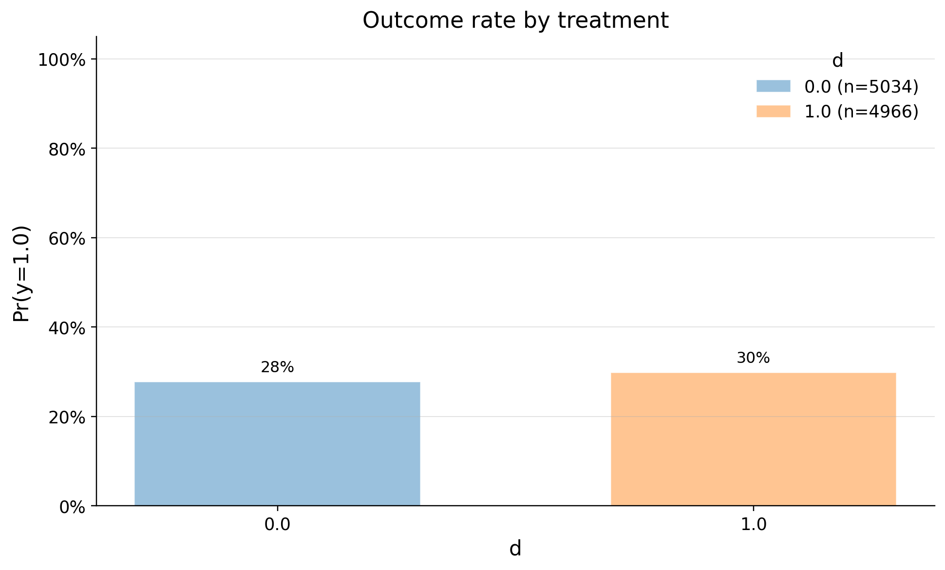
So we see that new section has higher conversion rate. Let's check if it is statistically significant and our test holds the indentification assumptions

Monitoring of the split

Result

SRMResult(status=no SRM, p_value=0.49650, chi2=0.4624)

Result

	confounders	mean_d_0	mean_d_1	abs_diff	smd	ks_pvalue
0	region_eu	0.210369	0.189086	0.021284	-0.053250	0.20331
1	spend_last_month	77.921167	75.111595	2.809573	-0.039381	0.68313
2	plan_tier_pro	0.151569	0.161095	0.009526	0.026230	0.97481
3	support_tickets	1.817839	1.789569	0.028270	-0.020930	0.72761
4	referral_count	0.797378	0.785139	0.012239	-0.013696	1.00000
5	tenure_months	13.780500	13.732216	0.048284	-0.006523	0.69284
6	plan_tier_plus	0.298967	0.296214	0.002753	-0.006020	1.00000
7	discount_rate	0.100375	0.100514	0.000139	0.002123	0.34966
8	y_pre	-0.000064	0.000065	0.000129	0.000612	0.64056
9	email_open_rate	0.447786	0.447805	0.000020	0.000155	0.95826

There is no evidence of breaking unconfoundedness assumption

Inference

We will use the CUPEDModel that implements the Lin (2013) "interacted adjustment" for ATE (Average Treatment Effect) estimation in randomized controlled trials (RCTs). This method is a robust version of ANCOVA that remains valid even when the treatment effect is heterogeneous with respect to the covariates.

1. Specification

The model fits an Ordinary Least Squares (OLS) regression of the outcome $Y$ on the treatment indicator $D$ and centered pre-treatment covariates $X^c$ . The specification includes full interactions between the treatment and the centered covariates:

$Y_i = \alpha + \tau D_i + \beta^T X_i^c + \gamma^T (D_i \cdot X_i^c) + \epsilon_i$

Where:

$Y_i$ : Outcome for individual $i$ .
$D_i$ : Binary treatment indicator ( $D_i \in \{0, 1\}$ ).
$X_i$ : Vector of pre-treatment covariates.
$X_i^c = X_i - \bar{X}$ : Centered covariates (where $\bar{X}$ is the sample mean).
$\alpha$ : Intercept (represents the mean outcome of the control group when $X = \bar{X}$ ).
$\tau$ : Average Treatment Effect (ATE) or Intent-to-Treat (ITT) effect.
$\beta$ : Vector of coefficients for the main effects of the covariates.
$\gamma$ : Vector of coefficients for the interaction terms between treatment and covariates.
$\epsilon_i$ : Residual error term.

Result

	value
field
estimand	ATE
model	CUPEDModel
value	0.0210 (ci_abs: 0.0054, 0.0365)
value_relative	7.5747 (ci_rel: 1.9572, 13.1923)
alpha	0.0500
p_value	0.0081
is_significant	True
n_treated	4966
n_control	5034
treatment_mean	0.2980
control_mean	0.2769
time	2026-02-18

Our result is significant with relative ci 7.5747% (ci_rel: 1.9572%, 13.1923%)

Result

png

Result

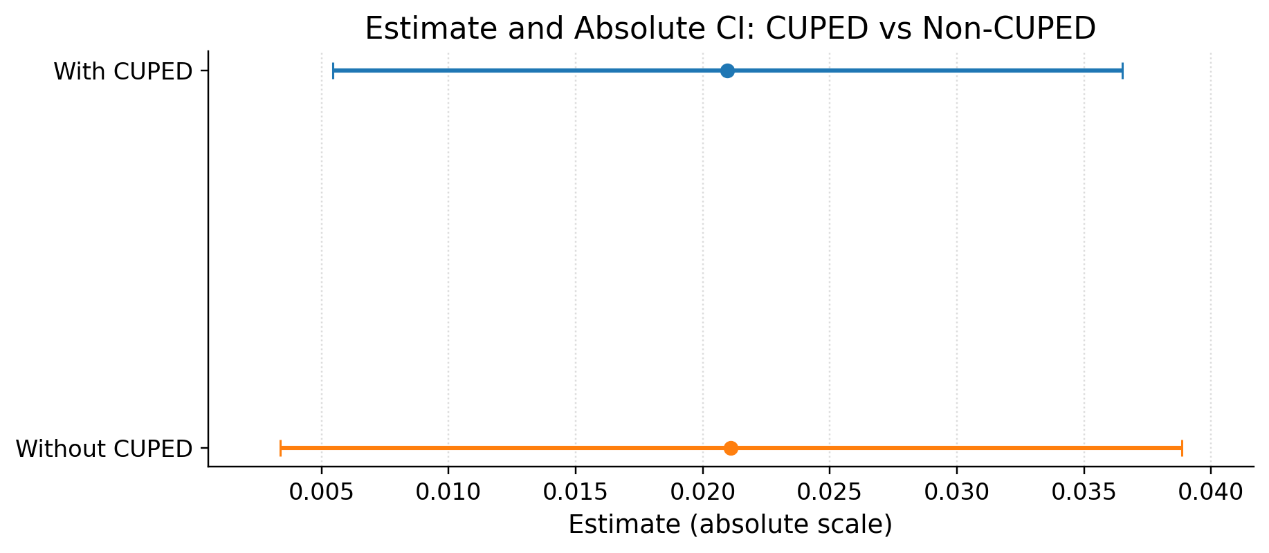
var reduction by CUPED %: 23.382355917736007

CUPED is worked. We reduced variance

Let's check other assuptions

SUTVA

Result

1.) Are your clients independent (i). Outcome of ones do not depend on others? 2.) Are all clients have full window to measure metrics? 3.) Do you measure confounders before treatment and outcome after? 4.) Do you have a consistent label of treatment, such as if a person does not receive a treatment, he has a label 0?

We assume that there is no networking effect
Metrics are valid
Confounders and covariates meseared before the treatment and outcome after
Lebeling treatment are consistent based of our logging system

Overlap

Overlap is true by design

Regression specification

Result

	test_id	test	flag	value	threshold	message
0	design_rank	Design rank	GREEN	rank=4, k=4	rank == k	Design matrix is full rank.
1	condition_number	Condition number	GREEN	12.310161	<= 1.000e+08	Condition number is within expected range.
2	near_duplicates	Near-duplicate covariates	GREEN	0	0 pairs	No near-duplicate centered covariates found.
3	vif	Variance inflation factor	GREEN	nan	<= 20	VIF not applicable (fewer than two usable covariates).
4	ate_gap	Adjusted vs naive ATE	GREEN	0.014799	yellow: > 2.00, red: > 2.50	Adjusted and naive ATE are reasonably aligned.
5	residual_tails	Residual extremes	GREEN	max\|std resid\|=2.53	yellow > 7, red > 10	Residual extremes look reasonable.
6	leverage	Leverage	GREEN	max_h=0.002482, n_high=787	yellow if max_h > 50.0008, red if max_h > max(0.5, 100.0008)	No high-leverage concentration detected.
7	cooks	Cook's distance	GREEN	max=0.003232, n_high=434	yellow if max Cook's > 0.1, red if > 1	No strong influence signal from Cook's distance.
8	hc23_stability	HC2/HC3 stability	GREEN	min(1-h)=9.975e-01, n_tiny=0	min(1-h) >= 1.0e-06	HC2/HC3 stability check passed.
9	winsor_sensitivity	Winsor sensitivity	GREEN	0.000000	yellow: > 1.00 SE, red: > 2.00 SE	Winsorized refit is close to baseline ATE.

Our regression specification is valid

In conclution

The new section is performing better than the older. Effect is "0.0210 (ci_abs: 0.0054, 0.0365)" in p.p. Roll out to all users