generate_cuped_binary_26
This notebook presents the generate cuped binary research workflow and key analysis steps.
The make_cuped_binary_26 data generating process (DGP) creates a synthetic binary-outcome dataset with randomized treatment, richer confounders, structured heterogeneous treatment effects (HTE), and a calibrated pre-period covariate (y_pre) for CUPED benchmarking.
1. Confounders
The DGP uses mixed-type confounders sampled from independent marginals:
tenure_months():spend_last_month():discount_rate():support_tickets():email_open_rate():referral_count():plan_tier(): Categorical with levelsfree(55%),plus(30%),pro(15%), encoded asplan_tier_plusandplan_tier_pro.region(): Categorical with levelsna(80%),eu(20%), encoded asregion_eu.
2. Treatment Assignment
Treatment is randomized with constant propensity: This is implemented with and no - or latent-driven treatment terms.
3. Outcome Model
The outcome is binary with a logistic link:
- .
- is a shared latent prognostic signal used only in the outcome equation (so treatment remains randomized/unconfounded).
- when
add_pre=True, and otherwise. - Baseline score combines monotone transformations of confounders and segment indicators.
4. Heterogeneous Treatment Effect
Treatment effect is defined on the log-odds scale: Where:
- by default.
5. Pre-period Covariate
If add_pre=True, first define a centered probability-scale baseline signal:
Then construct:
The noise scale is calibrated numerically so that in the control group matches the target correlation (default ).
| y | d | tenure_months | spend_last_month | discount_rate | support_tickets | email_open_rate | referral_count | plan_tier_plus | plan_tier_pro | region_eu | m | m_obs | tau_link | g0 | g1 | cate | y_pre | |
|---|---|---|---|---|---|---|---|---|---|---|---|---|---|---|---|---|---|---|
| 0 | 0.0 | 0.0 | 14.187461 | 62.867015 | 0.087395 | 2.0 | 0.412214 | 2.0 | 0.0 | 0.0 | 0.0 | 0.5 | 0.5 | 0.081508 | 0.267699 | 0.280682 | 0.012983 | 0.009942 |
| 1 | 0.0 | 0.0 | 7.242801 | 112.089626 | 0.173939 | 2.0 | 0.131957 | 0.0 | 0.0 | 0.0 | 0.0 | 0.5 | 0.5 | 0.037301 | 0.223180 | 0.228483 | 0.005303 | -0.220081 |
| 2 | 1.0 | 1.0 | 17.729423 | 16.813523 | 0.141900 | 2.0 | 0.376393 | 0.0 | 1.0 | 0.0 | 0.0 | 0.5 | 0.5 | 0.060442 | 0.245717 | 0.254861 | 0.009144 | 0.096021 |
| 3 | 0.0 | 0.0 | 19.497424 | 43.456545 | 0.146694 | 2.0 | 0.680602 | 1.0 | 0.0 | 0.0 | 0.0 | 0.5 | 0.5 | 0.096195 | 0.269024 | 0.284422 | 0.015398 | 0.188115 |
| 4 | 0.0 | 0.0 | 4.592766 | 105.987656 | 0.112326 | 6.0 | 0.642113 | 0.0 | 1.0 | 0.0 | 1.0 | 0.5 | 0.5 | 0.011141 | 0.264030 | 0.265771 | 0.001741 | -0.250511 |
Ground truth ATE is 0.011857450138243646 Ground truth ATTE is 0.011877088659875997
CausalData(df=(10000, 12), treatment='d', outcome='y', confounders=['tenure_months', 'spend_last_month', 'discount_rate', 'support_tickets', 'email_open_rate', 'referral_count', 'plan_tier_plus', 'plan_tier_pro', 'region_eu', 'y_pre'])
| treatment | count | mean | std | min | p10 | p25 | median | p75 | p90 | max | |
|---|---|---|---|---|---|---|---|---|---|---|---|
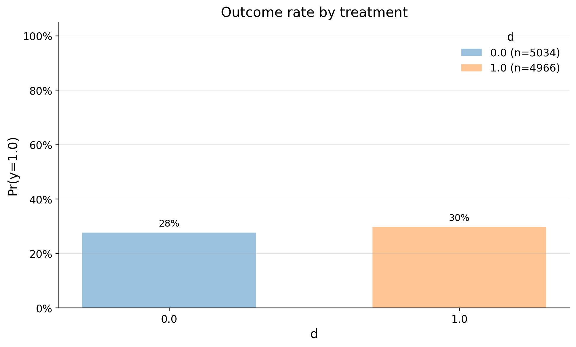
| 0 | 0.0 | 5034 | 0.276917 | 0.447520 | 0.0 | 0.0 | 0.0 | 0.0 | 1.0 | 1.0 | 1.0 |
| 1 | 1.0 | 4966 | 0.298027 | 0.457437 | 0.0 | 0.0 | 0.0 | 0.0 | 1.0 | 1.0 | 1.0 |
| confounders | mean_d_0 | mean_d_1 | abs_diff | smd | ks_pvalue | |
|---|---|---|---|---|---|---|
| 0 | region_eu | 0.210369 | 0.189086 | 0.021284 | -0.053250 | 0.20331 |
| 1 | spend_last_month | 77.921167 | 75.111595 | 2.809573 | -0.039381 | 0.68313 |
| 2 | plan_tier_pro | 0.151569 | 0.161095 | 0.009526 | 0.026230 | 0.97481 |
| 3 | support_tickets | 1.817839 | 1.789569 | 0.028270 | -0.020930 | 0.72761 |
| 4 | referral_count | 0.797378 | 0.785139 | 0.012239 | -0.013696 | 1.00000 |
| 5 | tenure_months | 13.780500 | 13.732216 | 0.048284 | -0.006523 | 0.69284 |
| 6 | plan_tier_plus | 0.298967 | 0.296214 | 0.002753 | -0.006020 | 1.00000 |
| 7 | discount_rate | 0.100375 | 0.100514 | 0.000139 | 0.002123 | 0.34966 |
| 8 | y_pre | -0.000064 | 0.000065 | 0.000129 | 0.000612 | 0.64056 |
| 9 | email_open_rate | 0.447786 | 0.447805 | 0.000020 | 0.000155 | 0.95826 |