Multi Unconfoundedness

Multi Unconfoundedness is observational/quasi experimental scenario of causal inference with multiple treatments. Treatments are not randomly assigned so we need to control confounders to estimate causal effect

Data

In our research we should estimate effect of different gamification mechanics. Our outcome is number of sessions per month.

Treatments:

d_0: No mechanics used
d_1: Used first set of mechanics
d_2: Used second set of mechanics

DGP is from Causalis. Read more at https://causalis.causalcraft.com/articles/generate_multitreatment_gamma_26

Result

	y	d_0	d_1	d_2	tenure_months	avg_sessions_week	spend_last_month	urban_resident	support_tickets_q	...	m_obs_d_1	tau_link_d_1	m_d_2	m_obs_d_2	tau_link_d_2	g_d_0	g_d_1	g_d_2	cate_d_1	cate_d_2
0	0.422769	1.0	0.0	0.0	27.656605	3.198667	89.609464	1.0	0.0	...	0.246687	-0.352005	0.220781	0.220781	0.494166	3.279384	2.306314	5.375338	-0.973070	2.095954
1	7.566231	1.0	0.0	0.0	23.798386	3.362415	102.337236	0.0	3.0	...	0.179393	-0.307360	0.236958	0.236958	0.420278	2.807850	2.064853	4.274630	-0.742997	1.466780
2	1.702662	0.0	0.0	1.0	28.425009	3.391819	102.660712	1.0	1.0	...	0.210566	-0.320189	0.218245	0.218245	0.502415	3.069919	2.228798	5.073677	-0.841121	2.003758
3	1.827530	1.0	0.0	0.0	18.860066	4.071175	83.593417	0.0	2.0	...	0.176729	-0.316241	0.237639	0.237639	0.441677	2.716805	1.980234	4.225485	-0.736571	1.508680
4	1.429843	0.0	1.0	0.0	17.853087	3.140075	79.209870	1.0	1.0	...	0.232492	-0.350130	0.247027	0.247027	0.493624	3.224354	2.271869	5.282273	-0.952485	2.057919

5 rows × 26 columns

Result

Ground truth ATE for d_1 vs d_0 is -1.1950325692907122 Ground truth ATE for d_2 vs d_0 is 2.530398527003894

Result

MultiCausalData(df=(100000, 12), treatment_names=['d_0', 'd_1', 'd_2'], control_treatment='d_0')outcome='y', confounders=['tenure_months', 'avg_sessions_week', 'spend_last_month', 'premium_user', 'urban_resident', 'support_tickets_q', 'discount_eligible', 'credit_utilization'], user_id=None,

EDA

Result

	treatment	count	mean	std	min	p10	p25	median	p75	p90	max
0	d_0	50115	3.758417	3.106725	0.015427	0.887906	1.626326	2.937863	4.957415	7.577785	50.239323
1	d_2	25008	6.541717	5.539708	0.043125	1.512610	2.775637	5.102611	8.584913	13.348761	79.125235
2	d_1	24877	2.980817	2.412763	0.009022	0.711997	1.306774	2.352234	3.946463	5.985070	25.169272

Result

png

Result

png

Result

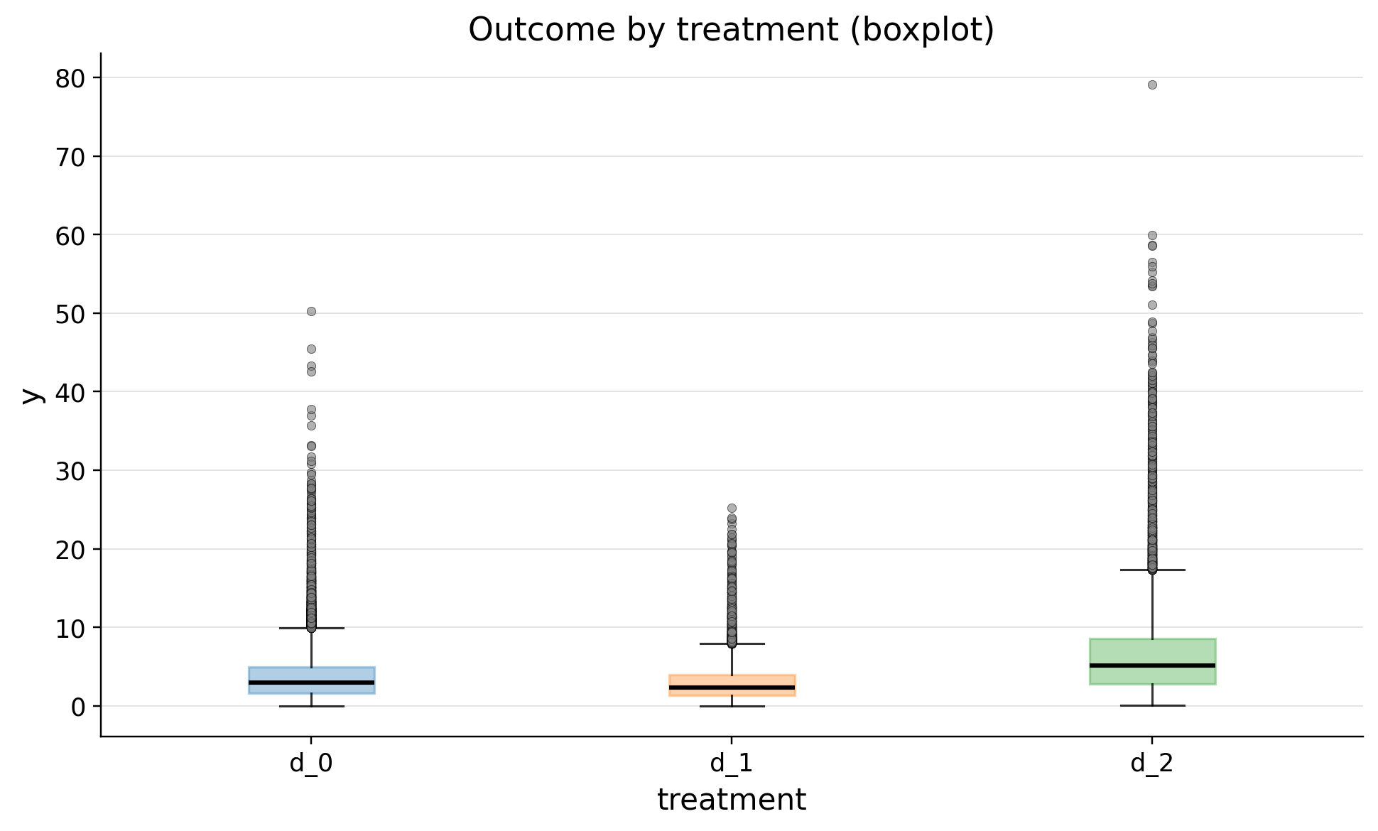
	treatment	n	outlier_count	outlier_rate	lower_bound	upper_bound	has_outliers	method	tail
0	d_0	50115	2288	0.045655	-3.370308	9.954048	True	iqr	both
1	d_2	25008	1173	0.046905	-5.938277	17.298826	True	iqr	both
2	d_1	24877	1067	0.042891	-2.652760	7.905997	True	iqr	both

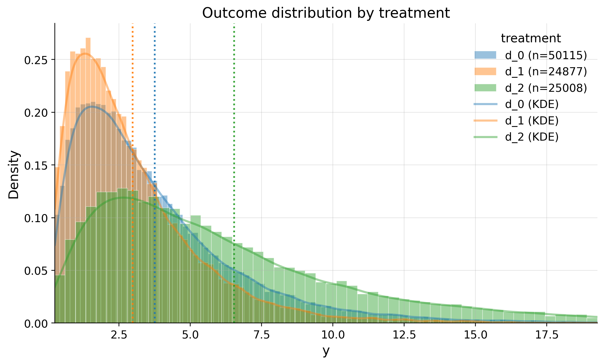
As we see there are heavy tails in distribution of outcome. We won't trim them because high activity means high income of revenue for us

Result

	confounders	mean_d_0	mean_d_1	abs_diff	smd	ks_pvalue
0	avg_sessions_week	4.827957	5.330050	0.502092	0.253187	0.00000
1	premium_user	0.217440	0.296861	0.079421	0.182466	0.00000
2	tenure_months	23.672462	25.752063	2.079601	0.176703	0.00000
3	spend_last_month	82.894719	96.062898	13.168180	0.149709	0.00000
4	discount_eligible	0.325870	0.395626	0.069756	0.145642	0.00000
5	urban_resident	0.585912	0.638421	0.052509	0.107919	0.00000
6	support_tickets_q	1.478140	1.492302	0.014162	0.011558	0.47358
7	credit_utilization	0.449627	0.448996	0.000632	-0.005811	0.86692

Result

	confounders	mean_d_0	mean_d_1	abs_diff	smd	ks_pvalue
0	premium_user	0.217440	0.274072	0.056632	0.131823	0.00000
1	avg_sessions_week	4.827957	5.059494	0.231536	0.116747	0.00000
2	spend_last_month	82.894719	89.334021	6.439302	0.076205	0.00000
3	support_tickets_q	1.478140	1.569378	0.091238	0.073883	0.00000
4	discount_eligible	0.325870	0.356006	0.030136	0.063605	0.00000
5	urban_resident	0.585912	0.604687	0.018774	0.038256	0.00002
6	tenure_months	23.672462	23.391337	0.281125	-0.024131	0.00373
7	credit_utilization	0.449627	0.451855	0.002228	0.020493	0.02836

And data is highly biased by confounders

Inference

Explanation of `MultiTreatmentIRM`

0) Assumptions

SUTVA / consistency: no interference, no hidden treatment versions, and observed outcome equals the potential outcome under realized arm.
Multi-arm unconfoundedness:

\left(Y(0),Y(1),\dots,Y(K-1)\right) \perp D \mid X

where $D$ is one-hot with baseline arm $D_0$ .

Positivity / overlap:

\Pr(D_k=1\mid X=x)>0,\quad \forall k=0,\dots,K-1.

In practice, the implementation enforces stability with propensity trimming.

1) Data and estimand

For each unit $i$ we observe $Y_i, X_i, D_i$ with one-hot $D_i=(D_{i0},\dots,D_{i,K-1})$ and $\sum_k D_{ik}=1$ .

MultiTreatmentIRM estimates vector contrasts against baseline:

\theta_k = \mathbb{E}[Y(k)-Y(0)],\quad k=1,\dots,K-1.

So outputs are pairwise ATEs such as d_1 vs d_0, d_2 vs d_0.

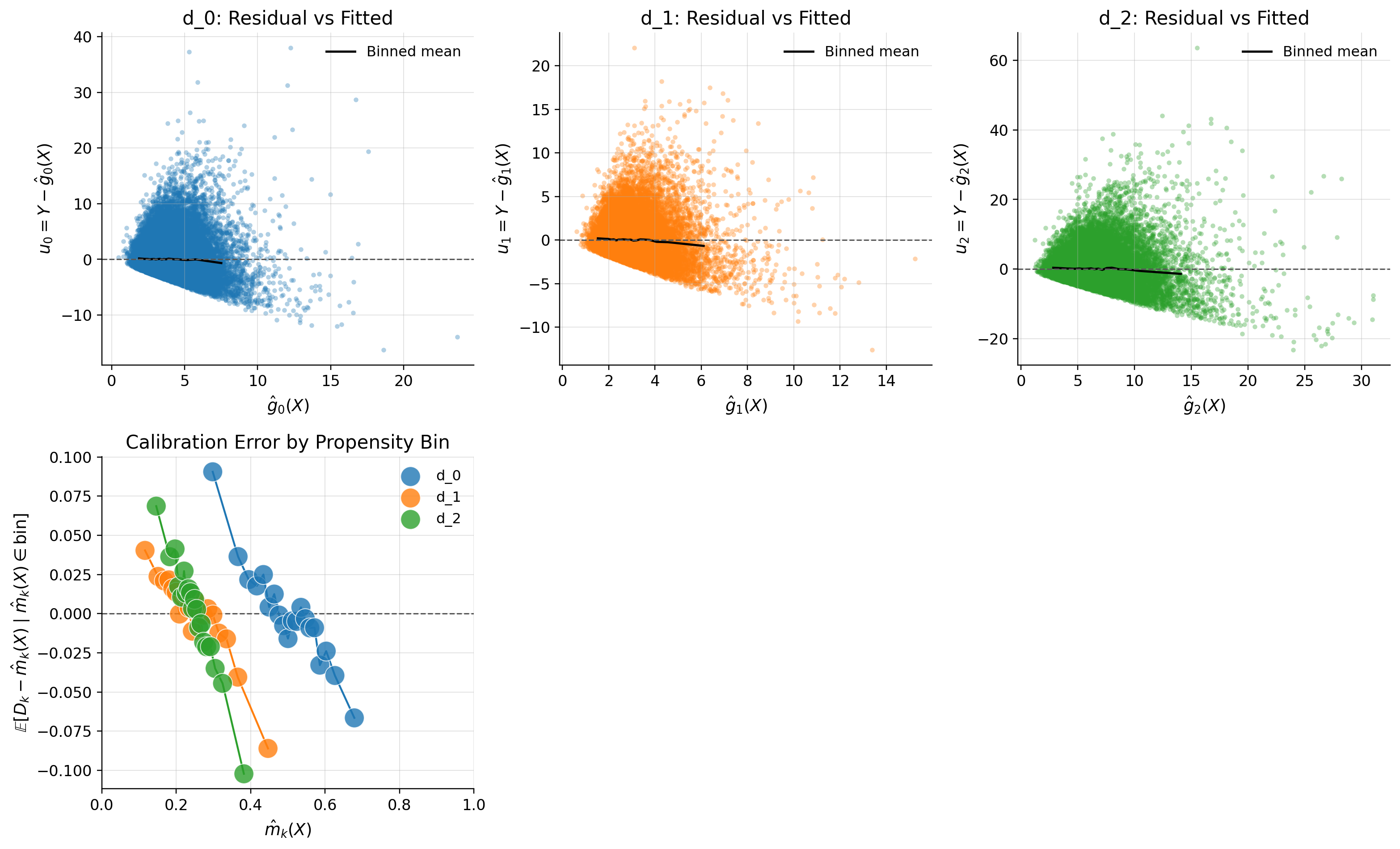
2) Nuisance functions

For each arm $k$ :

g_k(x)=\mathbb{E}[Y\mid X=x, D_k=1],\qquad m_k(x)=\Pr(D_k=1\mid X=x),\ \sum_{k=0}^{K-1}m_k(x)=1.

These are estimated out-of-fold by cross-fitting (to reduce overfitting bias in final moments).

3) Cross-fitting logic

With folds $I_1,\dots,I_F$ :

Train multiclass propensity model on $I_f^c$ , predict $\hat m_k$ on $I_f$ .
For each arm $k$ , train outcome model on rows in $I_f^c$ where $D_k=1$ , predict $\hat g_k$ on $I_f$ .
Repeat for all folds and stitch predictions.

4) Multiclass trimming

Predicted propensities are stabilized by lower-bound trimming and row renormalization:

\tilde m_{ik}=\max(\hat m_{ik},\varepsilon),\qquad \hat m^{trim}_{ik}=\frac{\tilde m_{ik}}{\sum_{j=0}^{K-1}\tilde m_{ij}}.

This keeps each row on the probability simplex and avoids exploding IPW weights.

5) Orthogonal score for each contrast

Define residuals and IPW representers:

u_{ik}=Y_i-\hat g_k(X_i),\qquad h_{ik}=\frac{D_{ik}}{\hat m^{trim}_{ik}}.

(If normalize_ipw=True, $h_{ik}$ is column-normalized in Hajek style.)

For each active arm $k>0$ vs baseline $0$ :

\psi_{b,ik}=\big(\hat g_k(X_i)-\hat g_0(X_i)\big)+u_{ik}h_{ik}-u_{i0}h_{i0}, \qquad \psi_a=-1.

Moment condition:

\mathbb{E}_n[\psi_a\theta_k+\psi_{b,\cdot k}]=0 \ \Rightarrow\ \hat\theta_k=\mathbb{E}_n[\psi_{b,\cdot k}].

6) Inference

Influence function per contrast:

\widehat{IF}_{ik}=\psi_{b,ik}-\hat\theta_k.

Then

\widehat{SE}(\hat\theta_k)=\sqrt{\frac{\mathrm{Var}_n(\widehat{IF}_{\cdot k})}{n}},

with Wald CI

\hat\theta_k \pm z_{1-\alpha/2}\widehat{SE}(\hat\theta_k).

P-values are normal-approximation; significance flag is Bonferroni-adjusted across $K-1$ contrasts.

7) Relative effect reported by the model

Baseline mean is estimated via orthogonal signal:

\psi_{\mu_c,i}=\hat g_0(X_i)+u_{i0}h_{i0},\qquad \hat\mu_c=\mathbb{E}_n[\psi_{\mu_c}].

Relative effect (%):

\hat\tau_k^{rel}=100\cdot\frac{\hat\theta_k}{\hat\mu_c},

with CI from delta-method variance (as implemented in model.py).

Result

	d_1 vs d_0	d_2 vs d_0
field
estimand	ATE	ATE
model	MultiTreatmentIRM	MultiTreatmentIRM
value	-1.1832 (ci_abs: -1.2233, -1.1431)	2.5298 (ci_abs: 2.4565, 2.6031)
value_relative	-29.9638 (ci_rel: -30.8175, -29.1101)	64.0643 (ci_rel: 61.9680, 66.1606)
alpha	0.0500	0.0500
p_value	0.0000	0.0000
is_significant	True	True
n_treated	24877	25008
n_control	50115	50115
treatment_mean	2.9808	6.5417
control_mean	3.7584	3.7584
time	2026-02-22	2026-02-22

Refutation

Unconfoundedness

Result

	comparison	metric	value	flag
0	d_0 vs d_1	balance_max_smd	0.013307	GREEN
1	d_0 vs d_1	balance_frac_violations	0.0	GREEN
2	d_0 vs d_1	balance_pass	True	GREEN
3	d_0 vs d_2	balance_max_smd	0.004068	GREEN
4	d_0 vs d_2	balance_frac_violations	0.0	GREEN
5	d_0 vs d_2	balance_pass	True	GREEN
6	overall	balance_max_smd	0.013307	GREEN
7	overall	balance_frac_violations	0.0	GREEN
8	overall	balance_pass	True	GREEN

Sensitivity

Result

	cf_y	r2_y	r2_d	rho	theta_long	theta_short	delta
d_1 vs d_0	3.022036e-07	3.022035e-07	1.351745e-07	-1.0	-1.183219	-1.146914	-0.036304
d_2 vs d_0	3.022036e-07	3.022035e-07	1.461506e-07	-1.0	2.529790	2.470708	0.059082

Result

{'theta': array([-1.18321853, 2.52979027]), 'se': array([0.02044409, 0.03741762]), 'alpha': 0.05, 'z': 1.959963984540054, 'H0': 0.0, 'sampling_ci': array([[-1.22328822, -1.14314885], [ 2.45645308, 2.60312746]]), 'theta_bounds_cofounding': array([[-1.61866521, -0.74777186], [ 2.1016666 , 2.95791394]]), 'bias_aware_ci': array([[-1.65985899, -0.70803275], [ 2.02990876, 3.03312867]]), 'max_bias_base': array([8.48841832, 8.34566666]), 'max_bias': array([0.43544667, 0.42812367]), 'bound_width': array([0.43544667, 0.42812367]), 'sigma2': 11.79593879649448, 'nu2': array([6.10830955, 5.90458744]), 'rv': array([0.27985187, 0.64760316]), 'rva': array([0.26617826, 0.63406235]), 'contrast_labels': ['d_1 vs d_0', 'd_2 vs d_0'], 'params': {'cf_y': 0.05, 'r2_d': array([0.05, 0.05]), 'rho': array([1., 1.]), 'use_signed_rr': False}}

Overlap

Result

png

Result

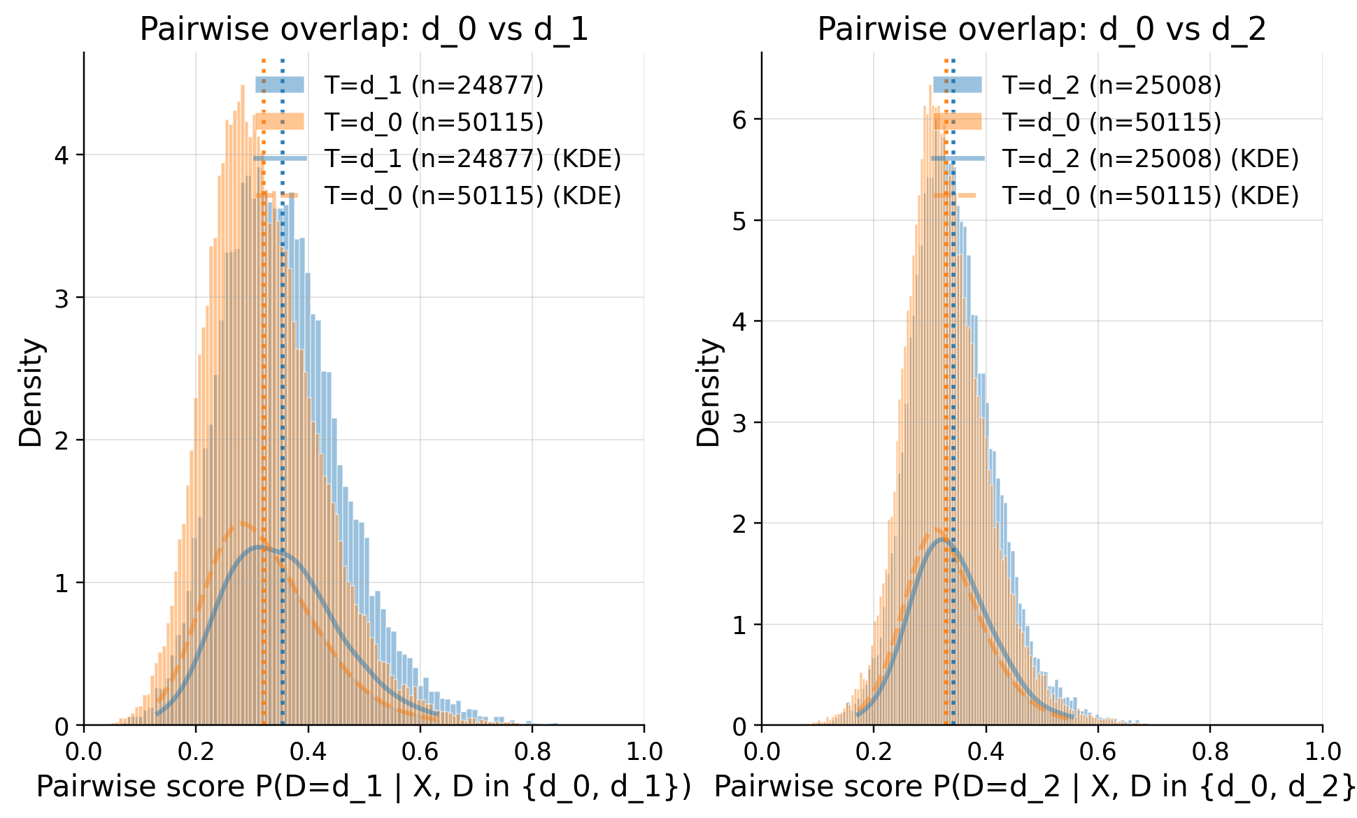
	comparison	metric	value	flag
0	d_0 vs d_1	edge_0.01_below	0.0	GREEN
1	d_0 vs d_1	edge_0.01_above	0.0	GREEN
2	d_0 vs d_1	KS	0.141067	GREEN
3	d_0 vs d_1	AUC	0.596814	GREEN
4	d_0 vs d_1	ESS_treated_ratio	0.895799	GREEN
5	d_0 vs d_1	ESS_baseline_ratio	0.954377	GREEN
6	d_0 vs d_1	clip_m_total	0.0	GREEN
7	d_0 vs d_1	overlap_pass	True	GREEN
8	d_0 vs d_2	edge_0.01_below	0.0	GREEN
9	d_0 vs d_2	edge_0.01_above	0.0	GREEN
10	d_0 vs d_2	KS	0.074956	GREEN
11	d_0 vs d_2	AUC	0.549007	GREEN
12	d_0 vs d_2	ESS_treated_ratio	0.948692	GREEN
13	d_0 vs d_2	ESS_baseline_ratio	0.954377	GREEN
14	d_0 vs d_2	clip_m_total	0.0	GREEN
15	d_0 vs d_2	overlap_pass	True	GREEN

SUTVA

Result

1.) Are your clients independent (i). Outcome of ones do not depend on others? 2.) Are all clients have full window to measure metrics? 3.) Do you measure confounders before treatment and outcome after? 4.) Do you have a consistent label of treatment, such as if a person does not receive a treatment, he has a label 0?

Score

Result

	comparison	metric	value	flag
0	d_1 vs d_0	se_plugin	2.044409e-02	NA
1	d_1 vs d_0	psi_p99_over_med	9.656081e+00	GREEN
2	d_1 vs d_0	psi_kurtosis	6.103705e+01	RED
3	d_1 vs d_0	max_\|t\|_gk	5.488800e+00	RED
4	d_1 vs d_0	max_\|t\|_g0	4.107007e+00	RED
5	d_1 vs d_0	max_\|t\|_mk	1.723246e+00	RED
6	d_1 vs d_0	max_\|t\|_m0	9.548751e-01	RED
7	d_1 vs d_0	max_\|t\|	5.488800e+00	RED
8	d_1 vs d_0	oos_tstat_fold	-1.028761e-15	GREEN
9	d_1 vs d_0	oos_tstat_strict	-1.779456e-15	GREEN
10	d_2 vs d_0	se_plugin	3.741762e-02	NA
11	d_2 vs d_0	psi_p99_over_med	1.610667e+01	YELLOW
12	d_2 vs d_0	psi_kurtosis	5.568245e+01	RED
13	d_2 vs d_0	max_\|t\|_gk	5.333558e+00	RED
14	d_2 vs d_0	max_\|t\|_g0	4.107007e+00	RED
15	d_2 vs d_0	max_\|t\|_mk	1.431120e+00	RED
16	d_2 vs d_0	max_\|t\|_m0	9.548751e-01	RED
17	d_2 vs d_0	max_\|t\|	5.333558e+00	RED
18	d_2 vs d_0	oos_tstat_fold	-4.861275e-16	GREEN
19	d_2 vs d_0	oos_tstat_strict	-6.684270e-16	GREEN

Result

png

Conclusion

Set of mechanics labeled d_2 performed better and has effect 2.5355 (ci_abs: 2.4600, 2.6111) sessions per user. However, set of mechanics labeled d_1 perform worse than without mechanics -1.1772 (ci_abs: -1.2174, -1.1370) sessions. We need to turn them off

Multi Unconfoundedness

Multi Unconfoundedness

Data

EDA

Inference

Explanation of MultiTreatmentIRM

0) Assumptions

1) Data and estimand

2) Nuisance functions

3) Cross-fitting logic

4) Multiclass trimming

5) Orthogonal score for each contrast

6) Inference

7) Relative effect reported by the model

Refutation

Unconfoundedness

Sensitivity

Overlap

SUTVA

Score

Conclusion

Explanation of `MultiTreatmentIRM`