generate_multitreatment_gamma_26()
This notebook presents the generate multitreatment gamma 26 research workflow and key analysis steps.
generate_multitreatment_gamma_26() builds a 3-arm multi-treatment observational DGP with correlated confounders and a Gamma outcome.
Treatment columns are one-hot: with exactly one active class per row (d_0, d_1, d_2).
The scenario is configured to target marginal treatment shares close to .
1. Confounders and Dependence
The confounder vector is with marginals:
- (
tenure_months) , clipped to - (
avg_sessions_week) , clipped to - (
spend_last_month) , clipped at 500 - (
premium_user) - (
urban_resident) - (
support_tickets_q) , clipped at 15 - (
discount_eligible) - (
credit_utilization) with mean and concentration
Dependence is induced with a Gaussian copula whose correlation matrix is Toeplitz:
2. Treatment Assignment (Multinomial Logit)
For each class , define score Then propensity is softmax:
Coefficients used in this scenario:
Treatment-score intercepts start at , then are calibrated iteratively so mean class rates are close to target .
3. Treatment Effects on Link Scale
The structural link shift for class is
Control has no heterogeneous residual: .
For d_1 (forced harmful vs control):
For d_2 (forced beneficial vs control):
4. Outcome Model (Gamma)
Baseline linear predictor: with
Observed link for assigned treatment:
Gamma mean uses log link: Given shape , outcome is sampled as so and .
5. Oracle Quantities
When include_oracle=True, the generator exposes:
m_d_0,m_d_1,m_d_2: calibrated propensitiestau_link_d_k: link-scale treatment shiftsg_d_k: potential outcome means on natural scale under classcate_d_1 = g_{d_1}-g_{d_0},cate_d_2 = g_{d_2}-g_{d_0}
| y | d_0 | d_1 | d_2 | tenure_months | avg_sessions_week | spend_last_month | premium_user | urban_resident | support_tickets_q | ... | m_obs_d_1 | tau_link_d_1 | m_d_2 | m_obs_d_2 | tau_link_d_2 | g_d_0 | g_d_1 | g_d_2 | cate_d_1 | cate_d_2 | |
|---|---|---|---|---|---|---|---|---|---|---|---|---|---|---|---|---|---|---|---|---|---|
| 0 | 0.422769 | 1.0 | 0.0 | 0.0 | 27.656605 | 3.198667 | 89.609464 | 0.0 | 1.0 | 0.0 | ... | 0.246687 | -0.352005 | 0.220781 | 0.220781 | 0.494166 | 3.279384 | 2.306314 | 5.375338 | -0.973070 | 2.095954 |
| 1 | 7.566231 | 1.0 | 0.0 | 0.0 | 23.798386 | 3.362415 | 102.337236 | 0.0 | 0.0 | 3.0 | ... | 0.179393 | -0.307360 | 0.236958 | 0.236958 | 0.420278 | 2.807850 | 2.064853 | 4.274630 | -0.742997 | 1.466780 |
| 2 | 1.702662 | 0.0 | 0.0 | 1.0 | 28.425009 | 3.391819 | 102.660712 | 0.0 | 1.0 | 1.0 | ... | 0.210566 | -0.320189 | 0.218245 | 0.218245 | 0.502415 | 3.069919 | 2.228798 | 5.073677 | -0.841121 | 2.003758 |
| 3 | 1.827530 | 1.0 | 0.0 | 0.0 | 18.860066 | 4.071175 | 83.593417 | 0.0 | 0.0 | 2.0 | ... | 0.176729 | -0.316241 | 0.237639 | 0.237639 | 0.441677 | 2.716805 | 1.980234 | 4.225485 | -0.736571 | 1.508680 |
| 4 | 1.429843 | 0.0 | 1.0 | 0.0 | 17.853087 | 3.140075 | 79.209870 | 0.0 | 1.0 | 1.0 | ... | 0.232492 | -0.350130 | 0.247027 | 0.247027 | 0.493624 | 3.224354 | 2.271869 | 5.282273 | -0.952485 | 2.057919 |
5 rows × 26 columns
Ground truth ATE for d_1 vs d_0 is -1.1950325692907122 Ground truth ATE for d_2 vs d_0 is 2.530398527003894
MultiCausalData(df=(100000, 12), treatment_names=['d_0', 'd_1', 'd_2'], control_treatment='d_0')outcome='y', confounders=['tenure_months', 'avg_sessions_week', 'spend_last_month', 'premium_user', 'urban_resident', 'support_tickets_q', 'discount_eligible', 'credit_utilization'], user_id=None,
| treatment | count | mean | std | min | p10 | p25 | median | p75 | p90 | max | |
|---|---|---|---|---|---|---|---|---|---|---|---|
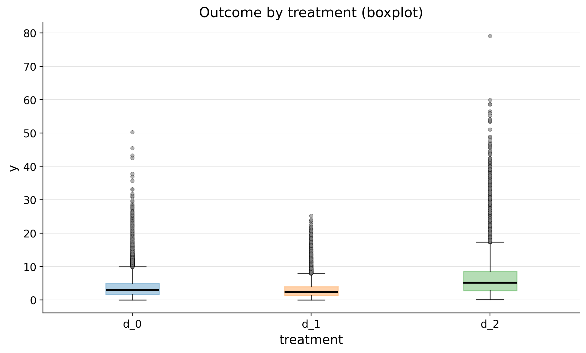
| 0 | d_0 | 50115 | 3.758417 | 3.106725 | 0.015427 | 0.887906 | 1.626326 | 2.937863 | 4.957415 | 7.577785 | 50.239323 |
| 1 | d_2 | 25008 | 6.541717 | 5.539708 | 0.043125 | 1.512610 | 2.775637 | 5.102611 | 8.584913 | 13.348761 | 79.125235 |
| 2 | d_1 | 24877 | 2.980817 | 2.412763 | 0.009022 | 0.711997 | 1.306774 | 2.352234 | 3.946463 | 5.985070 | 25.169272 |

| treatment | n | outlier_count | outlier_rate | lower_bound | upper_bound | has_outliers | method | tail | |
|---|---|---|---|---|---|---|---|---|---|
| 0 | d_0 | 50115 | 2288 | 0.045655 | -3.370308 | 9.954048 | True | iqr | both |
| 1 | d_2 | 25008 | 1173 | 0.046905 | -5.938277 | 17.298826 | True | iqr | both |
| 2 | d_1 | 24877 | 1067 | 0.042891 | -2.652760 | 7.905997 | True | iqr | both |
| confounders | mean_d_0 | mean_d_1 | abs_diff | smd | ks_pvalue | |
|---|---|---|---|---|---|---|
| 0 | premium_user | 0.217440 | 0.274072 | 0.056632 | 0.131823 | 0.00000 |
| 1 | avg_sessions_week | 4.827957 | 5.059494 | 0.231536 | 0.116747 | 0.00000 |
| 2 | spend_last_month | 82.894719 | 89.334021 | 6.439302 | 0.076205 | 0.00000 |
| 3 | support_tickets_q | 1.478140 | 1.569378 | 0.091238 | 0.073883 | 0.00000 |
| 4 | discount_eligible | 0.325870 | 0.356006 | 0.030136 | 0.063605 | 0.00000 |
| 5 | urban_resident | 0.585912 | 0.604687 | 0.018774 | 0.038256 | 0.00002 |
| 6 | tenure_months | 23.672462 | 23.391337 | 0.281125 | -0.024131 | 0.00373 |
| 7 | credit_utilization | 0.449627 | 0.451855 | 0.002228 | 0.020493 | 0.02836 |
| confounders | mean_d_0 | mean_d_1 | abs_diff | smd | ks_pvalue | |
|---|---|---|---|---|---|---|
| 0 | avg_sessions_week | 4.827957 | 5.330050 | 0.502092 | 0.253187 | 0.00000 |
| 1 | premium_user | 0.217440 | 0.296861 | 0.079421 | 0.182466 | 0.00000 |
| 2 | tenure_months | 23.672462 | 25.752063 | 2.079601 | 0.176703 | 0.00000 |
| 3 | spend_last_month | 82.894719 | 96.062898 | 13.168180 | 0.149709 | 0.00000 |
| 4 | discount_eligible | 0.325870 | 0.395626 | 0.069756 | 0.145642 | 0.00000 |
| 5 | urban_resident | 0.585912 | 0.638421 | 0.052509 | 0.107919 | 0.00000 |
| 6 | support_tickets_q | 1.478140 | 1.492302 | 0.014162 | 0.011558 | 0.47358 |
| 7 | credit_utilization | 0.449627 | 0.448996 | 0.000632 | -0.005811 | 0.86692 |