CUPED

We call 'Controlled-experiment Using Pre-Experiment Data' (CUPED) a scenario where a treatment is randomly assigned to participants, and we have pre-experiment data of participants like pre-treatment outcome.

Treatment - new product category for users.

We will test hypothesis:

$H_o$ - There is no difference in LTV between treatment and control groups.

$H_a$ - There is a difference in LTV between treatment and control groups.

Causal Assumptions

Unconfoundedness: random assignment of treatment. Will be tested with SRM and Balance Check

Overlap: each unit has a non-zero probability of assignment to every arm. By design

SUTVA: no interference and consistent treatment definitions. By design

Pre-treatment covariate: exists and predicts outcome

Data

For the analysis you need data in pandas dataframe:

treatment column in binary format (1/0)
outcome column numeric format, measured after treatment time
user_id column (Optional, but useful)
confounders columns (Optional, measured before treatment time, numeric format, used for causal assumption check, includes covariates for CUPED)

We will take data from Causalis DGP. Read more at https://causalis.causalcraft.com/articles/make_cuped_tweedie_26

Result

	y	d	tenure_months	avg_sessions_week	spend_last_month	discount_rate	platform_ios	m	m_obs	tau_link	g0	g1	cate	y_pre	_latent_A	y_pre_2
0	3.734763	0.0	14.187461	2.0	57.355300	0.158164	1.0	0.5	0.5	0.103825	8.487966	9.416605	0.928639	17.972138	0.304717	10.783283
1	0.746406	1.0	6.352893	3.0	46.700946	0.085722	0.0	0.5	0.5	0.030781	8.487966	8.753301	0.265335	0.000000	-1.039984	0.000000
2	13.040584	1.0	18.910153	9.0	80.136187	0.175115	1.0	0.5	0.5	0.357355	8.487966	12.133915	3.645949	34.771837	0.750451	24.866330
3	34.582113	1.0	7.927627	4.0	33.718224	0.152718	1.0	0.5	0.5	0.065554	8.487966	9.063025	0.575059	349.163943	0.940565	209.498366
4	0.000000	1.0	11.106925	2.0	92.064518	0.077390	0.0	0.5	0.5	0.056036	8.487966	8.977172	0.489206	0.000000	-1.951035	0.243980

Result

CausalData(df=(20000, 9), treatment='d', outcome='y', confounders=['avg_sessions_week', 'spend_last_month', 'discount_rate', 'platform_ios', 'platform_web', 'y_pre', 'y_pre_2'])

EDA

Result

	treatment	count	mean	std	min	p10	p25	median	p75	p90	max
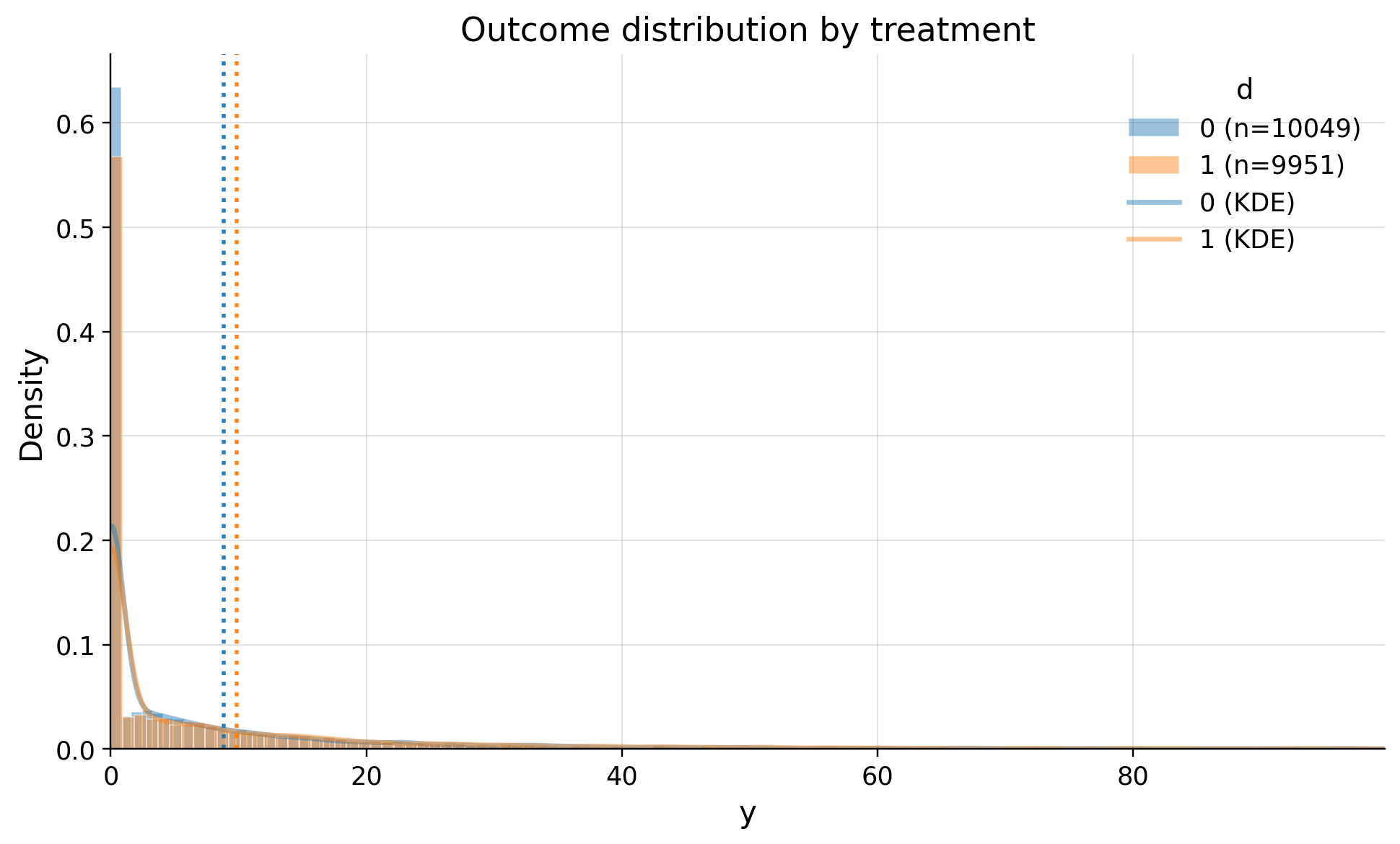
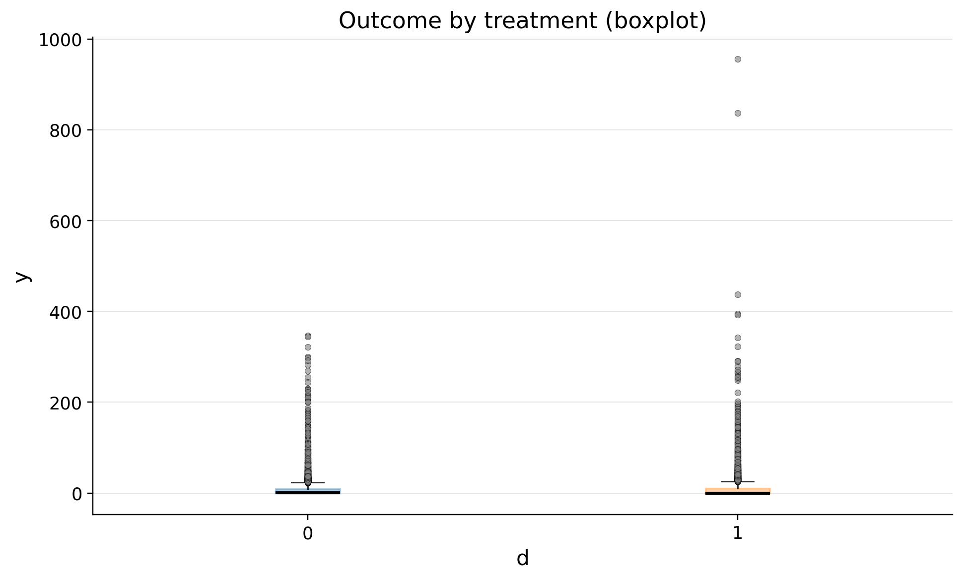
0	0	10049	8.867136	21.097599	0.0	0.0	0.0	0.276901	9.266134	24.454852	347.095992
1	1	9951	9.870188	25.879015	0.0	0.0	0.0	0.000000	10.409916	27.439125	956.413897

Result

png

Result

png

Result

	treatment	n	outlier_count	outlier_rate	lower_bound	upper_bound	has_outliers	method	tail
0	0	10049	1080	0.107473	-13.899201	23.165335	True	iqr	both
1	1	9951	1063	0.106823	-15.614875	26.024791	True	iqr	both

We see heavy tale distribution

SRM

Some system is randomly splitting users. Half must have new onboarding, other half has not. We should monitor the split with SRM test. Read more at https://causalis.causalcraft.com/articles/srm

Result

SRMResult(status=no SRM, p_value=0.48833, chi2=0.4802)

Confounders balance

Result

	confounders	mean_d_0	mean_d_1	abs_diff	smd	ks_pvalue
0	spend_last_month	73.787667	75.159017	1.371350	0.019726	0.20812
1	platform_ios	0.304309	0.297357	0.006952	-0.015158	0.96771
2	y_pre	7928.516448	20967.672427	13039.155979	0.014621	0.36084
3	y_pre_2	4760.192129	12583.709202	7823.517073	0.014621	0.38473
4	avg_sessions_week	4.963379	5.015677	0.052297	0.012405	0.49401
5	discount_rate	0.100420	0.099996	0.000424	-0.006421	0.36146
6	platform_web	0.050950	0.050749	0.000202	-0.000918	1.00000

SRM is good
SMD < 0.1 and ks_pvalue > 0.05

Split is random. Uncofoundedness is true

Inference with CUPED

Read more about model specification at https://causalis.causalcraft.com/articles/cuped-model

Result

	value
field
estimand	ATE
model	CUPEDModel
value	0.8155 (ci_abs: 0.2724, 1.3587)
value_relative	9.0633 (ci_rel: 2.7548, 15.3718)
alpha	0.0500
p_value	0.0033
is_significant	True
n_treated	9951
n_control	10049
treatment_mean	9.8702
control_mean	8.8671
time	2026-05-09

Refutation

Result

png

Result

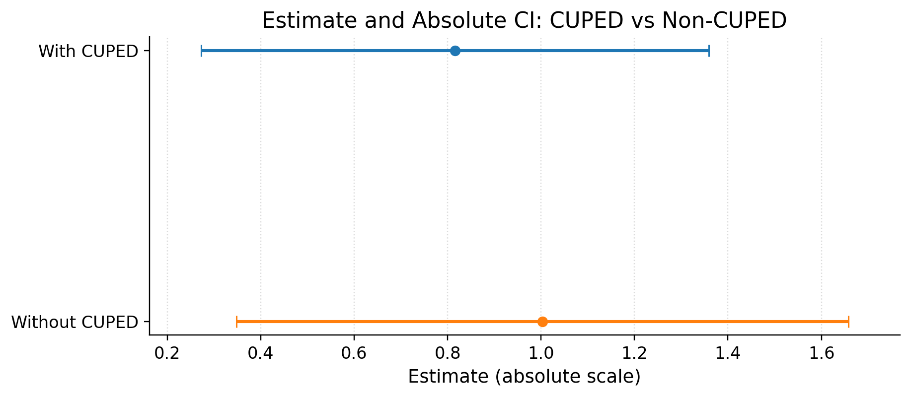
var reduction with CUPED %: 31.179489563275986

Result

	test_id	test	flag	value	threshold	message
0	design_rank	Design rank	GREEN	rank=6, k=6	rank == k	Design matrix is full rank.
1	condition_number	Condition number	GREEN	3335417.561613	<= 1.000e+08	Condition number is within expected range.
2	near_duplicates	Near-duplicate covariates	YELLOW	1	red if >= 3	Near-duplicate covariate pairs detected.
3	vif	Variance inflation factor	RED	6485299680.233781	yellow: > 20, red: > 40	Very large VIF indicates severe multicollinearity.
4	ate_gap	Adjusted vs naive ATE	GREEN	0.561334	yellow: > 2.00, red: > 2.50	Adjusted and naive ATE are reasonably aligned.
5	residual_tails	Residual extremes	RED	max\|std resid\|=27.8	yellow > 7, red > 10	Extremely large standardized residuals; outliers likely dominate.
6	leverage	Leverage	RED	max_h=0.91, n_high=653	yellow if max_h > 50.0006, red if max_h > max(0.5, 100.0006)	Extreme leverage points detected.
7	cooks	Cook's distance	RED	max=1301, n_high=778	yellow if max Cook's > 0.1, red if > 1	Strongly influential observations detected.
8	hc23_stability	HC2/HC3 stability	GREEN	min(1-h)=9.004e-02, n_tiny=0	min(1-h) >= 1.0e-06	HC2/HC3 stability check passed.
9	winsor_sensitivity	Winsor sensitivity	GREEN	0.304010	yellow: > 1.00 SE, red: > 2.00 SE	Winsorized refit is close to baseline ATE.

let's compare it to oracle effect

Result

Ground truth ATE is 1.2383515933360814