The make_cuped_tweedie_26 data generating process (DGP) creates a synthetic dataset characterized by a Tweedie-like outcome (zero-inflated with a heavy right tail), correlated confounders, and structured heterogeneous treatment effects (HTE). It also includes a pre-period covariate (y_pre) calibrated for CUPED benchmarks.
1. Confounders ()
Five confounders are generated using a Gaussian Copula to induce specific correlations:
tenure_months():avg_sessions_week():spend_last_month():discount_rate():platform(): Categorical with levelsandroid(65%),ios(30%),web(5%).
Correlations: and .
2. Treatment Assignment ()
The treatment is assigned via a Bernoulli trial with a constant propensity score (RCT):
(Note: While the generator supports complex propensity models, make_cuped_tweedie_26 defaults to a balanced random assignment).
3. Outcome Model ()
The outcome is generated as a two-part (hurdle) process:
A. Binary Indicator of Non-zero Outcome ()
- is the sigmoid function.
- (resulting in ~50% baseline non-zero rate).
- (if
add_pre=True). - is an unobserved confounder.
B. Positive Outcome Value ()
If , the value is drawn from a Gamma distribution:
- (shape parameter).
- , where is the linear predictor on the log-mean scale:
- .
- (if
add_pre=True).
4. Heterogeneous Treatment Effect ()
The treatment effect is defined on the log-mean scale and incorporates monotone effects, diminishing returns, and categorical modifiers: Where:
- (Saturating effect of tenure).
- (Diminishing returns of sessions).
- (Premium segment modifier).
- (Default log-uplift parameter).
5. Pre-period Covariate ()
The pre-period covariate is generated using the same two-part structure as the outcome but replaces the unobserved confounder with a shared latent driver :
- .
- The influence of the shared driver and the noise scale are calibrated (via numerical optimization) to ensure achieves a target correlation (default ) with the post-period outcome in the control group.
| y | d | tenure_months | avg_sessions_week | spend_last_month | discount_rate | platform_ios | platform_web | m | m_obs | tau_link | g0 | g1 | cate | y_pre | |
|---|---|---|---|---|---|---|---|---|---|---|---|---|---|---|---|
| 0 | 0.000000 | 0.0 | 14.187461 | 2.0 | 57.355300 | 0.158164 | 0.0 | 0.0 | 0.5 | 0.5 | 0.042035 | 3.694528 | 3.853136 | 0.158608 | 0.000000 |
| 1 | 0.000000 | 1.0 | 6.352893 | 3.0 | 46.700946 | 0.085722 | 0.0 | 0.0 | 0.5 | 0.5 | 0.016201 | 3.694528 | 3.754870 | 0.060342 | 0.000000 |
| 2 | 12.918910 | 0.0 | 18.910153 | 9.0 | 80.136187 | 0.175115 | 1.0 | 0.0 | 0.5 | 0.5 | 0.188082 | 3.694528 | 4.459044 | 0.764516 | 219.374863 |
| 3 | 13.079312 | 1.0 | 7.927627 | 4.0 | 33.718224 | 0.152718 | 0.0 | 0.0 | 0.5 | 0.5 | 0.026540 | 3.694528 | 3.793893 | 0.099365 | 0.000000 |
| 4 | 0.000000 | 0.0 | 11.106925 | 2.0 | 92.064518 | 0.077390 | 0.0 | 0.0 | 0.5 | 0.5 | 0.029492 | 3.694528 | 3.805111 | 0.110583 | 0.000000 |
Ground truth ATE is 0.2700720823988466 Ground truth ATTE is 0.27094666120202526
CausalData(df=(100000, 9), treatment='d', outcome='y', confounders=['tenure_months', 'avg_sessions_week', 'spend_last_month', 'discount_rate', 'platform_ios', 'platform_web', 'y_pre'])
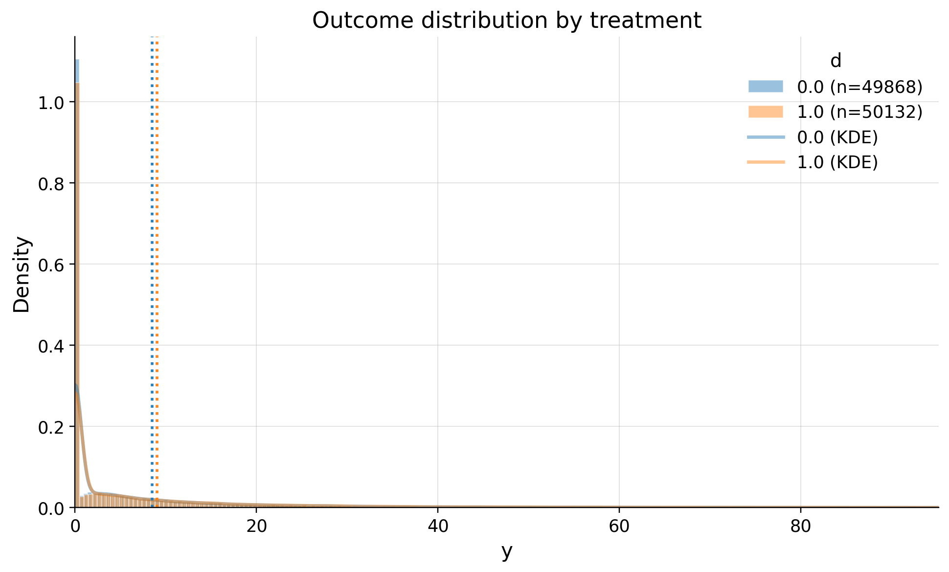
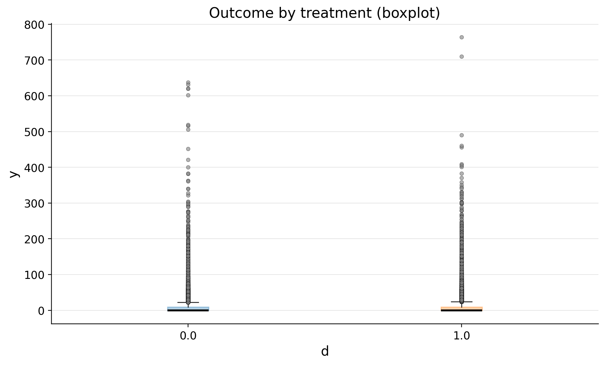
| treatment | count | mean | std | min | p10 | p25 | median | p75 | p90 | max | |
|---|---|---|---|---|---|---|---|---|---|---|---|
| 0 | 0.0 | 49868 | 8.496830 | 20.907555 | 0.0 | 0.0 | 0.0 | 0.0 | 8.903005 | 23.685134 | 637.127367 |
| 1 | 1.0 | 50132 | 9.056301 | 21.790102 | 0.0 | 0.0 | 0.0 | 0.0 | 9.523496 | 25.207978 | 764.333725 |
| confounders | mean_d_0 | mean_d_1 | abs_diff | smd | ks_pvalue | |
|---|---|---|---|---|---|---|
| 0 | platform_web | 0.051356 | 0.048312 | 0.003043 | -0.013985 | 0.97420 |
| 1 | y_pre | 15420.530166 | 51673.005274 | 36252.475108 | 0.008842 | 0.22562 |
| 2 | tenure_months | 13.756301 | 13.794400 | 0.038099 | 0.005198 | 0.56587 |
| 3 | platform_ios | 0.300032 | 0.301444 | 0.001412 | 0.003079 | 1.00000 |
| 4 | avg_sessions_week | 4.995969 | 5.003610 | 0.007641 | 0.001816 | 0.88605 |
| 5 | spend_last_month | 75.176560 | 75.263792 | 0.087232 | 0.001222 | 0.22678 |
| 6 | discount_rate | 0.100197 | 0.100129 | 0.000068 | -0.001031 | 0.64488 |