Uncofoundedness

We call 'Uncofoundedness' a scenario where a treatment is not randomly assigned to participants, so confounders effect on treatment assignment and outcome.

Treatment - purchase in one category.

We will test hypothesis:

$H_o$ - There is no difference in LTV between treatment and control groups.

$H_a$ - There is a difference in LTV between treatment and control groups.

Result

	y	d	tenure_months	avg_sessions_week	spend_last_month	age_years	income_monthly	prior_purchases_12m	support_tickets_90d	premium_user	mobile_user	urban_resident	referred_user	m	m_obs	tau_link	g0	g1	cate
0	0.000000	0.0	28.814654	1.0	77.936767	50.234101	1926.698301	1.0	2.0	1.0	1.0	1.0	0.0	0.047970	0.047970	1.330764	8.137981	35.177086	27.039105
1	559.364158	1.0	25.913345	3.0	53.777740	28.115859	5104.271509	3.0	0.0	1.0	1.0	0.0	1.0	0.049695	0.049695	2.190209	60.459257	584.580685	524.121427
2	26.143003	1.0	24.969929	10.0	134.764322	22.907062	5267.938255	8.0	3.0	0.0	1.0	1.0	0.0	0.077087	0.077087	1.570177	7.712855	38.297992	30.585137
3	19.283585	1.0	40.655089	5.0	59.517074	31.970490	6597.327018	3.0	2.0	1.0	1.0	1.0	0.0	0.069481	0.069481	1.933844	25.386510	189.737828	164.351318
4	0.000000	1.0	18.560899	3.0	74.370930	39.237248	4930.009628	5.0	1.0	1.0	1.0	0.0	0.0	0.047097	0.047097	1.818265	15.359250	102.433597	87.074347

Result

Ground truth ATE is 617.0712367740982 Ground truth ATTE is 837.4043605736649

Result

CausalData(df=(100000, 13), treatment='d', outcome='y', confounders=['tenure_months', 'avg_sessions_week', 'spend_last_month', 'age_years', 'income_monthly', 'prior_purchases_12m', 'support_tickets_90d', 'premium_user', 'mobile_user', 'urban_resident', 'referred_user'])

Result

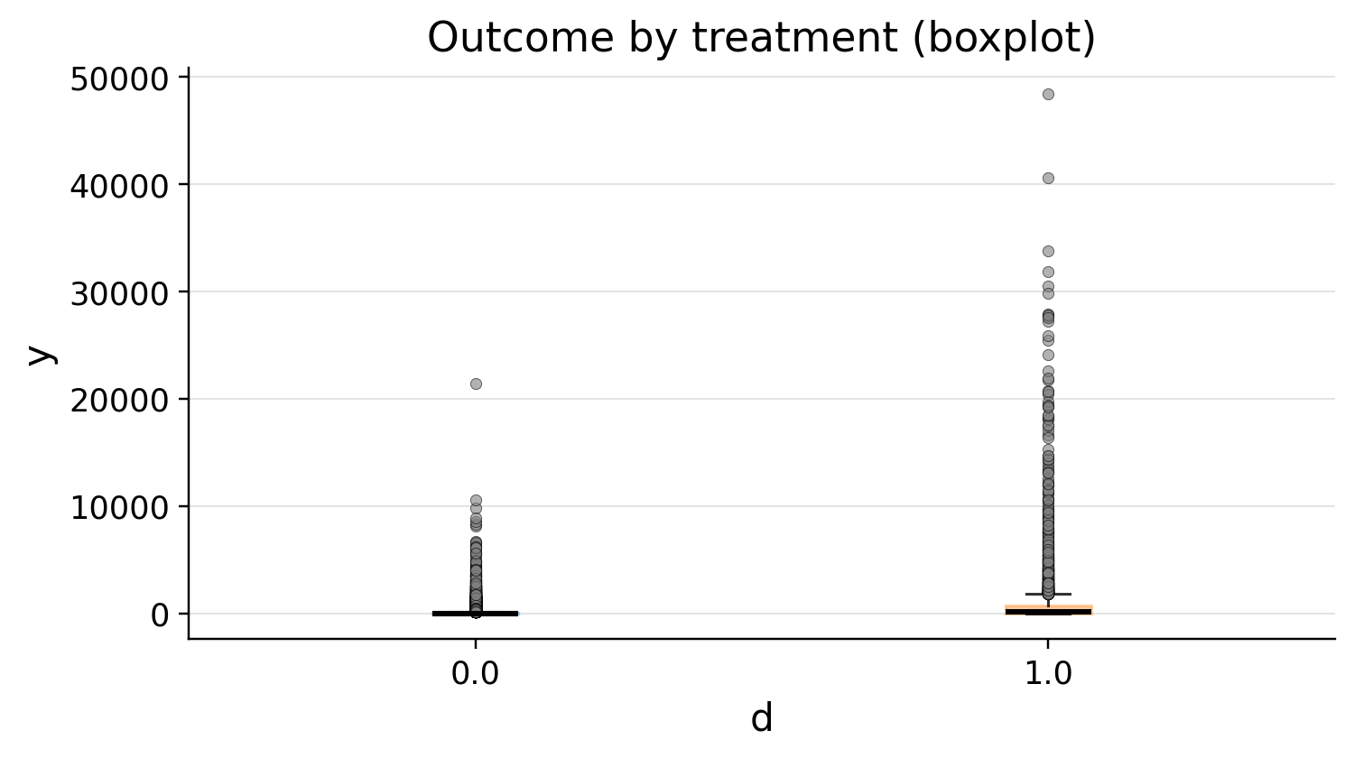
	treatment	count	mean	std	min	p10	p25	median	p75	p90	max
0	0.0	95015	73.966492	238.503707	0.0	0.0	0.0	7.448482	62.190137	184.701873	21396.007575
1	1.0	4985	907.471726	2545.077996	0.0	0.0	0.0	143.706288	730.651759	2269.458998	48466.747037

Result

png

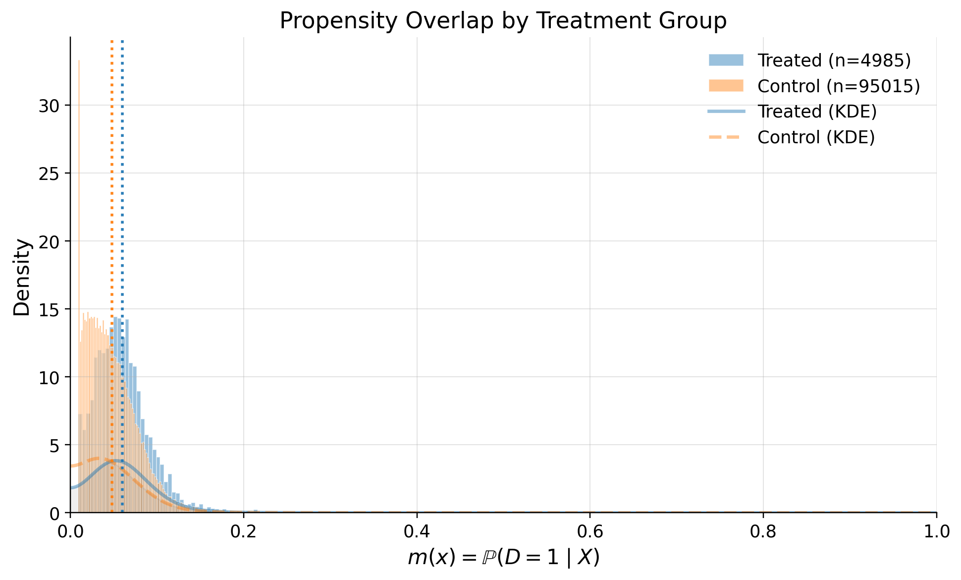
(<Figure size 1540x880 with 1 Axes>, <Figure size 1540x880 with 1 Axes>)

Result

	confounders	mean_d_0	mean_d_1	abs_diff	smd	ks_pvalue
0	spend_last_month	86.467107	117.559365	31.092259	0.329735	0.00000
1	avg_sessions_week	4.945293	6.188967	1.243674	0.287878	0.00000
2	premium_user	0.738199	0.852357	0.114158	0.285782	0.00000
3	prior_purchases_12m	3.863548	4.291675	0.428127	0.200809	0.00000
4	income_monthly	4496.964003	4921.775317	424.811314	0.169596	0.00000
5	age_years	36.446101	34.628006	1.818095	-0.162591	0.00000
6	referred_user	0.270599	0.323771	0.053172	0.116536	0.00000
7	mobile_user	0.872546	0.908726	0.036180	0.116115	0.00001
8	urban_resident	0.597169	0.638114	0.040945	0.084327	0.00000
9	support_tickets_90d	0.994138	1.074423	0.080286	0.077965	0.00002
10	tenure_months	28.523084	29.718502	1.195418	0.064588	0.00000

Inference

Math Explanation of the IRM Model and ATTE Estimand

The Interactive Regression Model (IRM) is a flexible framework used in Double Machine Learning (DML) to estimate treatment effects. Unlike linear models, it allows the treatment effect to vary with confounders $X$ (interaction) and makes no parametric assumptions about the functional forms of the outcomes.

We write $W=(Y,D,X)$ for an observation, where $D\in\{0,1\}$ is treatment and $Y$ is the observed outcome.

1. Nuisance Functions

The IRM framework relies on three "nuisance" components estimated from the data:

Outcome Regression (Control): $g_0(X) = \mathbb{E}[Y | X, D=0]$
Outcome Regression (Treated): $g_1(X) = \mathbb{E}[Y | X, D=1]$
Propensity Score: $m(X) = \mathbb{P}(D=1 | X)$

Let $p = \mathbb{P}(D=1) = \mathbb{E}[D]$ denote the overall treatment rate (estimated by the sample mean of $D$ ).

In the provided implementation (irm.py), these are estimated using cross-fitting (splitting data into folds) to avoid overfitting bias.

2. ATTE (Average Treatment Effect on the Treated)

The Average Treatment Effect on the Treated (ATTE) measures the impact of the treatment specifically on those individuals who received it: $\theta_{ATTE} = \mathbb{E}[Y(1) - Y(0) \mid D=1]$

Under unconfoundedness, $(Y(1),Y(0)) \perp D \mid X$ , and overlap $0 < m(X) < 1$ , this is identified from observed data.

3. The Orthogonal Score

DML uses a Neyman-orthogonal score $\psi$ to ensure the estimator is robust to small errors in the nuisance function estimates. The score for ATTE is defined as: $\psi(W; \theta, \eta) = \psi_b(W; \eta) + \psi_a(W; \eta)\theta$

To match the implementation in irm.py, define:

Residuals: $u_0 = Y - g_0(X)$ , $u_1 = Y - g_1(X)$
IPW terms: $h_1 = \frac{D}{m(X)}$ , $h_0 = \frac{1-D}{1-m(X)}$
Weights (ATTE): $w = \frac{D}{p}$ and $\bar{w} = \frac{m(X)}{p}$ (the normalized form with $\mathbb{E}[w]=1$ )

Then: \begin{aligned} \psi_a(W;\eta) &= -w = -\frac{D}{p} \ \psi_b(W;\eta) &= w,(g_1(X)-g_0(X)) + \bar{w},(u_1 h_1 - u_0 h_0) \end{aligned}

(If normalize_ipw=True, the code rescales $h_1$ and $h_0$ to have mean 1.)

4. Final Estimation (Step-by-step simplification)

For brevity, write $m = m(X)$ , $g_0 = g_0(X)$ , and $g_1 = g_1(X)$ . Plug in $w, \bar{w}, h_1, h_0$ :

\begin{aligned} \psi_b &= \frac{D}{p}(g_1-g_0)

\frac{m}{p}\left[\frac{D}{m}(Y-g_1) - \frac{1-D}{1-m}(Y-g_0)\right] \ &= \frac{D}{p}(g_1-g_0) + \frac{D}{p}(Y-g_1) - \frac{m}{p}\frac{1-D}{1-m}(Y-g_0) \ &= \frac{D}{p}(Y-g_0) - \frac{m}{p}\frac{1-D}{1-m}(Y-g_0). \end{aligned}

So the $g_1(X)$ terms cancel, and the ATTE score depends only on $g_0(X)$ and $m(X)$ .

The estimator solves $\mathbb{E}[\psi(W;\theta,\eta)]=0$ : \begin{aligned} \hat{\theta}_{ATTE} &= \frac{\mathbb{E}[\psi_b]}{\mathbb{E}[-\psi_a]} = \frac{\mathbb{E}[\psi_b]}{\mathbb{E}[D/p]} = \mathbb{E}[\psi_b]. \end{aligned}

Equivalently, $\hat{\theta}_{ATTE} = \mathbb{E}\left[\frac{D}{p}(Y-g_0(X)) - \frac{m(X)}{p}\frac{1-D}{1-m(X)}(Y-g_0(X))\right].$

Result

	estimand	coefficient	p_val	lower_ci	upper_ci	relative_diff_%	is_significant
0	ATTE	816.966741	0.0	749.154822	884.77866	893.17824	True

Result

CausalEstimate(estimand='ATTE', model='IRM', model_options={'n_folds': 5, 'n_rep': 1, 'normalize_ipw': False, 'trimming_rule': 'truncate', 'trimming_threshold': 0.01, 'random_state': None, 'std_error': 34.59855341330873, 't_stat': 23.61274273910593}, value=816.9667408936743, ci_upper_absolute=884.7786595009447, ci_lower_absolute=749.1548222864039, value_relative=893.1782401420442, ci_upper_relative=967.3160563964027, ci_lower_relative=819.0404238876857, alpha=0.05, p_value=0.0, is_significant=True, n_treated=4985, n_control=95015, outcome='y', treatment='d', confounders=['tenure_months', 'avg_sessions_week', 'spend_last_month', 'age_years', 'income_monthly', 'prior_purchases_12m', 'support_tickets_90d', 'premium_user', 'mobile_user', 'urban_resident', 'referred_user'], time=datetime.datetime(2026, 1, 27, 8, 26, 46, 441822), diagnostic_data=UnconfoundednessDiagnosticData(m_hat=array([0.05620082, 0.06597108, 0.12947216, ..., 0.03993944, 0.06856774, 0.0686461 ], shape=(100000,)), d=array([0, 1, 1, ..., 0, 0, 0], shape=(100000,)), y=array([ 0. , 559.3641575 , 26.14300299, ..., 86.88646582, 169.67753671, 0. ], shape=(100000,)), x=array([[ 28.81465403, 1. , 77.9367668 , ..., 1. ,

, 0. ], [ 25.91334462, 3. , 53.7777399 , ..., 1. ,
, 1. ], [ 24.9699287 , 10. , 134.76432201, ..., 1. ,
, 0. ], ..., [ 18.95058854, 2. , 49.18443354, ..., 1. ,
, 0. ], [ 22.87615781, 6. , 46.8461344 , ..., 1. ,
, 1. ], [ 38.81380133, 4. , 149.87138917, ..., 1. ,
, 1. ]], shape=(100000, 11)), g0_hat=array([ -1.88039973, 70.12097778, -2.32580324, ..., 85.09028141, 219.30257652, 284.15408662], shape=(100000,)), g1_hat=array([ 3.52125899, 626.31094544, 255.36485828, ..., 556.25218828, 1510.46557774, 2935.52765031], shape=(100000,)), psi_b=array([-2.24619835e+00, 9.81430651e+03, 5.71089393e+02, ..., -1.49895669e+00, 7.32831695e+01, 4.20136010e+02], shape=(100000,)), folds=array([0, 1, 4, ..., 3, 2, 3], shape=(100000,)), trimming_threshold=0.01, sigma2=230611.39428973786, nu2=20.51450972522466, psi_sigma2=array([-230607.8583866 , -226129.52187451, -178068.73534978, ..., -230608.1680113 , -228148.74971339, -149867.84934463], shape=(100000,)), psi_nu2=array([ 25.98365281, -366.08026856, -303.22555781, ..., 12.27041473, 36.55198755, 36.61933817], shape=(100000,)), riesz_rep=array([-1.19453237, 20.06018054, 20.06018054, ..., -0.83452271, -1.47673775, -1.47854995], shape=(100000,)), m_alpha=array([23.96253506, 28.42254226, 59.84989764, ..., 16.74067631, 29.62362582, 29.65997892], shape=(100000,)), psi=array([-2.24619835e+00, -6.57419380e+03, -1.58174109e+04, ..., -1.49895669e+00, 7.32831695e+01, 4.20136010e+02], shape=(100000,)), score='ATTE'), sensitivity_analysis={})

Result

	metric	value	flag
0	edge_0.01_below	0.000000	GREEN
1	edge_0.01_above	0.000000	GREEN
2	edge_0.02_below	0.183620	RED
3	edge_0.02_above	0.000000	RED
4	KS	0.193386	GREEN
5	AUC	0.623803	GREEN
6	ESS_treated_ratio	0.639887	GREEN
7	ESS_control_ratio	0.998503	GREEN
8	tails_w1_q99/med	5.610889	GREEN
9	tails_w0_q99/med	1.307781	GREEN
10	ATT_identity_relerr	0.012851	GREEN
11	clip_m_total	0.049540	YELLOW
12	calib_ECE	0.006803	GREEN
13	calib_slope	0.626749	YELLOW
14	calib_intercept	-1.036712	RED

Result

png

Result

	metric	value	flag
0	se_plugin	34.598553	NA
1	psi_p99_over_med	828.340166	RED
2	psi_kurtosis	1769.053579	RED
3	max_\|t\|_g1	0.000000	GREEN
4	max_\|t\|_g0	0.872006	GREEN
5	max_\|t\|_m	0.417469	GREEN

Result

1.) Are your clients independent (i)? 2.) Do you measure confounders, treatment, and outcome in the same intervals? 3.) Do you measure confounders before treatment and outcome after? 4.) Do you have a consistent label of treatment, such as if a person does not receive a treatment, he has a label 0?

Result

	metric	value	flag
0	balance_max_smd	0.018554	GREEN
1	balance_frac_violations	0.000000	GREEN

Result

{'theta': 816.9667408936743, 'se': 34.59855341330873, 'alpha': 0.05, 'z': 1.959963984540054, 'H0': 0.0, 'sampling_ci': (749.1548222864039, 884.7786595009447), 'theta_bounds_cofounding': (794.9964525215009, 838.9370292658477), 'bias_aware_ci': (728.8783636080927, 908.4863956227268), 'max_bias': 21.97028837217341, 'sigma2': 230611.39428973786, 'nu2': 20.51450972522466, 'rv': 0.2730480733887724, 'rva': 0.2561902047512034, 'params': {'r2_y': 0.01, 'r2_d': 0.01, 'rho': 1.0, 'use_signed_rr': False}}

Result

	r2_y	r2_d	rho	theta_long	theta_short	delta
d	0.000261	0.000496	-1.0	816.966741	816.176488	0.790253