Instrumental Variables (IV)

In many scenarios, the treatment is not assigned randomly, and there are unobserved confounders that affect both the treatment and the outcome. In such cases, we can use an Instrumental Variable (IV) to estimate the Local Average Treatment Effect (LATE).

Causal Assumptions

First-stage strength: instruments must be strongly correlated with the treatment.

Reduced form: instrument must affect the outcome only through the treatment.

Instrument balance by Z: instrument should be as good as random, independent of confounders.

Instrument propensity / predictability: instrument assignment should not be perfectly predictable from observed confounders.

Subgroup first-stage stability

Correct time order: X before Z, Z before D, D before Y: by design

Data

For the analysis you need data in pandas dataframe:

treatment column in binary format (1/0)
outcome column numeric format, measured after treatment time
instruments column in binary format (1/0), measured before treatment time
user_id column (Optional, but useful)
confounders columns (Optional, measured before instrument time, numeric format, used for causal assumption check)

We will use the generate_offer_iv_26 DGP from causalis

Result

	user_id	net_revenue_90d	accepted_offer	offer_eligible	age	tenure_months	annual_income	credit_score	app_sessions_30d	prior_spend_30d	...	g_z0	g_z1	iv_first_stage	iv_reduced_form	late_x	late	tau_link	g_d0	g_d1	cate
0	030f6	48.279955	0.0	0.0	42.0	39.154939	31608.240102	608.0	8.0	135.193819	...	33.125526	37.110160	0.254016	3.984633	15.686553	16.939349	15.686553	31.032649	46.719202	15.686553
1	03f52	39.719108	0.0	0.0	37.0	32.736592	214134.071780	727.0	4.0	491.348038	...	80.788151	88.054619	0.330043	7.266468	22.016741	16.939349	22.016741	72.536790	94.553531	22.016741
2	02ba6	49.727505	0.0	0.0	55.0	21.023638	95958.504507	643.0	7.0	189.244171	...	54.183327	58.871145	0.295717	4.687818	15.852359	16.939349	15.852359	51.189302	67.041662	15.852359
3	02e17	72.155483	1.0	1.0	25.0	18.105017	35715.886364	617.0	11.0	187.196966	...	66.779471	74.938408	0.331056	8.158937	24.645154	16.939349	24.645154	57.819237	82.464391	24.645154
4	0443a	33.330021	0.0	0.0	19.0	62.996281	107316.360040	691.0	2.0	113.817846	...	50.285174	54.246284	0.286149	3.961110	13.842813	16.939349	13.842813	47.884921	61.727734	13.842813

5 rows × 30 columns

Result

IVCausalData(df=(20000, 16), treatment='accepted_offer', outcome='net_revenue_90d', instruments=['offer_eligible'], confounders=['age', 'tenure_months', 'annual_income', 'credit_score', 'app_sessions_30d', 'prior_spend_30d', 'savings_balance', 'premium_user', 'autopay_enabled', 'region_north', 'region_west', 'acquisition_paid'], user_id='user_id')

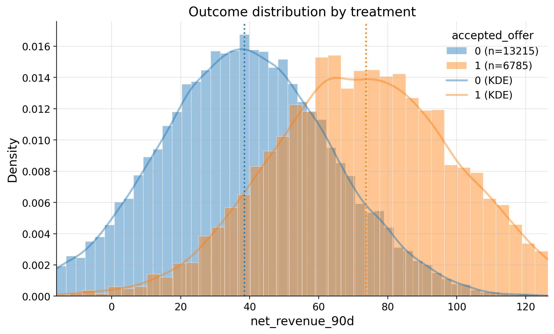
EDA

Result

	treatment	count	mean	std	min	p10	p25	median	p75	p90	max
0	0	13215	38.494730	25.145975	-49.067110	6.322963	21.665921	38.406990	55.429396	70.823578	137.335543
1	1	6785	73.709423	27.678527	-33.508289	38.841811	54.860868	73.235466	92.284659	109.586879	170.766350

Result

png

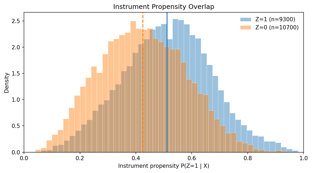
Check the confounders balance for the instrument

Are groups equal in terms of confounders? We check the balance of confounders across the instrument assignment (offer_eligible).

Result

	confounders	mean_z_0	mean_z_1	abs_diff	smd	ks_pvalue
0	credit_score	659.763925	693.257527	33.493602	0.532581	0.00000
1	annual_income	84199.971125	99330.828981	15130.857856	0.286549	0.00000
2	tenure_months	28.492666	32.022261	3.529595	0.180959	0.00000
3	autopay_enabled	0.357290	0.444624	0.087334	0.178902	0.00000
4	premium_user	0.241589	0.313763	0.072175	0.161675	0.00000
5	acquisition_paid	0.451963	0.377312	0.074651	-0.151955	0.00000
6	savings_balance	7027.452482	8913.472089	1886.019607	0.151898	0.00000
7	prior_spend_30d	156.527119	172.979941	16.452822	0.110804	0.00000
8	age	37.699533	38.662581	0.963048	0.087552	0.00000
9	app_sessions_30d	7.218411	7.526022	0.307610	0.072912	0.00018
10	region_north	0.208785	0.231613	0.022828	0.055107	0.01101
11	region_west	0.200093	0.198925	0.001169	-0.002924	1.00000

Inference

Result

IIVM(status='fitted', n_folds=5, random_state=None)

Result

	value
field
estimand	LATE
model	IIVM
value	19.1385 (ci_abs: 16.9702, 21.3068)
value_relative	None
std_error	1.1063
t_stat	17.2999
alpha	0.0500
p_value	0.0000
is_significant	True
outcome	net_revenue_90d
treatment	accepted_offer
instrument	offer_eligible
time	2026-05-10

Diagnostics

Result

	metric	value	flag	threshold	message
0	first_stage_effect	0.282397	GREEN	GREEN F >= 10; YELLOW 4 <= F < 10; RED F < 4 o...	Coefficient on Z in D ~ 1 + Z + X.
1	first_stage_se	0.006291	GREEN	GREEN when finite; RED when unavailable or inv...	HC1 robust standard error for the Z coefficient.
2	first_stage_pvalue	0.0	GREEN	GREEN when finite; RED when unavailable or inv...	HC1 robust p-value for the Z coefficient.
3	first_stage_f	2015.048215	GREEN	GREEN F >= 10; YELLOW 4 <= F < 10; RED F < 4 o...	Robust first-stage Wald F for the single instr...
4	partial_r2	0.095442	GREEN	GREEN when finite; RED when unavailable or inv...	Partial R-squared added by Z after controlling...
5	orthogonal_first_stage	0.281294	GREEN	GREEN F >= 10; YELLOW 4 <= F < 10; RED F < 4 o...	Denominator of the orthogonal LATE score.
6	weak_iv_flag	GREEN	GREEN	GREEN F >= 10; YELLOW 4 <= F < 10; RED F < 4 o...	First stage is strong enough for IV inference.

Result

	metric	value	flag	threshold	message
0	instrument_auc	0.653257	YELLOW	GREEN <0.60; YELLOW 0.60-0.75; RED >0.75 by ma...	How well covariates predict the instrument; hi...
1	instrument_propensity_ks	0.226303	GREEN	GREEN <=0.30; YELLOW >0.30-0.40; RED >0.40	Two-sample KS distance between Z=1 and Z=0 pro...
2	instrument_ess_ratio	0.813130	GREEN	GREEN >=0.30; YELLOW 0.15-0.30; RED <0.15	Minimum observed-arm IPW effective-sample-size...

Result

png

Result

	metric	value	flag	threshold	message
0	reduced_form_effect	1.076413e+01	GREEN	GREEN when finite; RED when unavailable or inv...	Coefficient on Z in Y ~ 1 + Z.
1	reduced_form_se	4.336784e-01	GREEN	GREEN when finite; RED when unavailable or inv...	HC1 robust standard error for the reduced-form...
2	reduced_form_pvalue	5.379896e-136	GREEN	GREEN when finite; RED when unavailable or inv...	HC1 robust p-value; non-significance is not a ...
3	orthogonal_reduced_form	5.383544e+00	GREEN	GREEN when finite; RED when unavailable or inv...	Numerator of the orthogonal LATE score.
4	late_ratio_check	1.913849e+01	GREEN	GREEN when finite; RED when unavailable or inv...	Orthogonal reduced form divided by orthogonal ...

Refutation

let's compare with oracle effect

Result

Ground truth LATE (oracle) is 16.939348789576744