generate_scm_gamma_26()

This notebook presents the generate scm gamma 26 research workflow and key analysis steps.

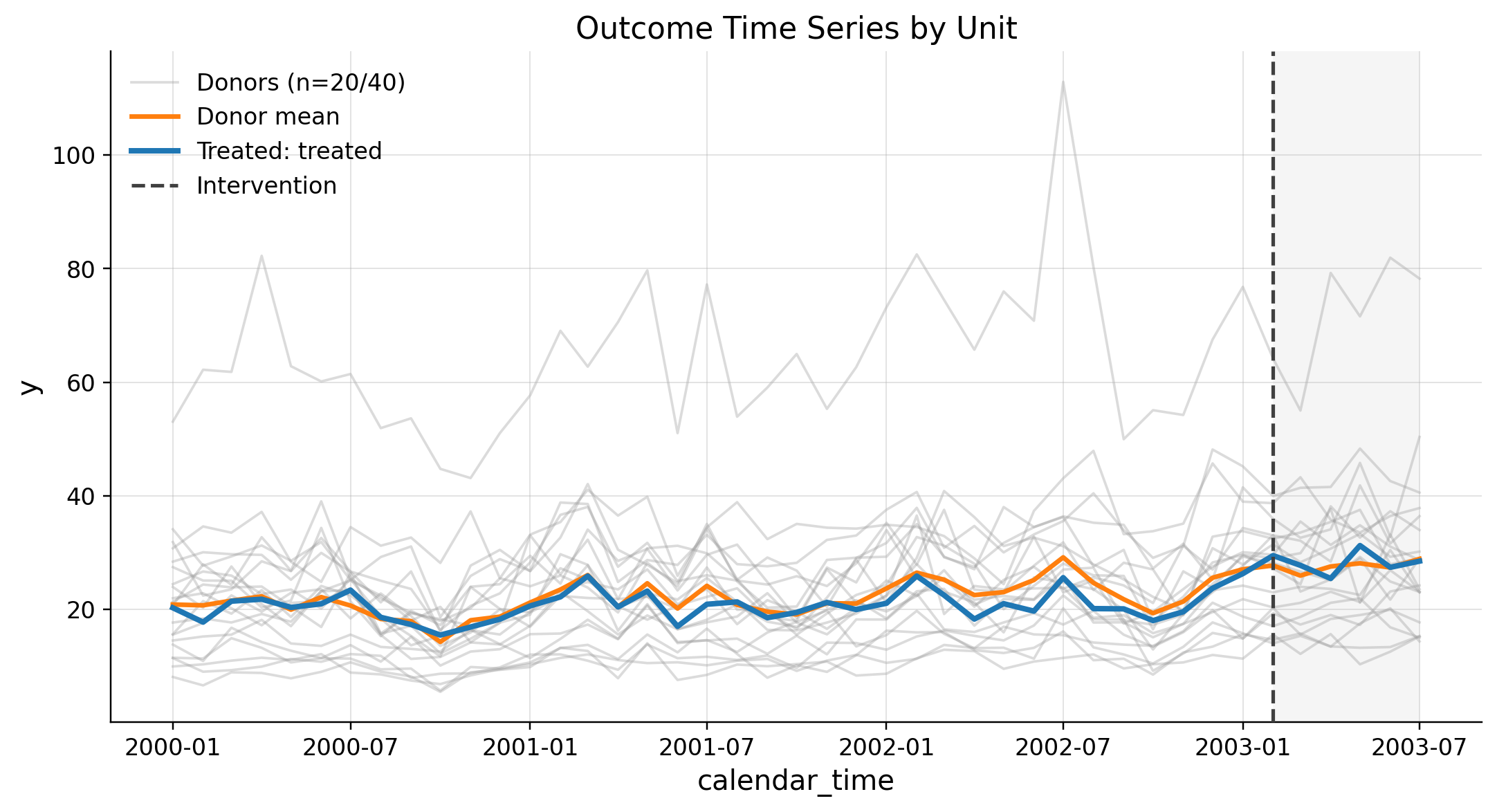
This scenario produces synthetic panel data with one treated unit and multiple donors. It uses a low-level Gamma DGP to simulate realistic outcomes with time-varying exposure and latent rates.

DGP math

The Data Generating Process (DGP) for the Gamma SCM scenario follows a hierarchical log-linear model for the mean $\mu$, with observations $y$ sampled from a Gamma distribution.

1.1 Donor units

For each donor unit $j$ at time $t$:

1. Exposure $E_{tj}$: $\log(E_{tj}) = \alpha_j + \gamma_j (t - \bar{t}) + \epsilon_t^{\text{common\_exp}} + \epsilon_{tj}^{\text{donor\_exp}}$ where $\epsilon_t^{\text{common\_exp}}$ and $\epsilon_{tj}^{\text{donor\_exp}}$ are AR(1) processes.
2. Mean $\mu_{tj}$: $\mu_{tj} = E_{tj} \cdot \exp(\eta_{tj})$ $\eta_{tj} = \beta_j + \delta_j (t - \bar{t}) + \lambda_j S_t + L_t + \sum_{k} \phi_{jk} F_{tk} + \epsilon_{tj}^{\text{donor\_noise}}$ where:
   • $S_t$: monthly seasonality signal
   • $L_t$: common factor (macro log index, AR(1))
   • $F_{tk}$: latent factors (AR(1))
   • $\epsilon_{tj}^{\text{donor\_noise}}$: donor-specific AR(1) noise
3. Outcome $y_{tj}$: $y_{tj} \sim \text{Gamma}\left(k, \frac{\mu_{tj}}{k}\right)$ where $k$ is the gamma_shape parameter.

1.2 Treated unit

The counterfactual mean $\mu_{t, cf}$ is a weighted combination of donors, potentially with a pre-fit mismatch: $\mu_{t, cf} = \left( \sum_j w_j \mu_{tj} \right) \cdot \exp(\epsilon_t^{\text{mismatch}})$ where $w \sim \text{Dirichlet}(\alpha)$.

Treatment is active only in post periods. For post step $k = 0,1,\dots,n_{post}-1$: $r_k = 1 - e^{-(k+1)/2.5}, \qquad \tau_k^{\text{rate}} = (\beta_0 + \beta_1 k)\,r_k$ where $\beta_0$ is treatment_effect_rate and $\beta_1$ is treatment_effect_slope.

Equivalently, in calendar time: $\tau_t^{\text{rate}} = 0 \text{ in pre/anchor periods, and } \tau_t^{\text{rate}} = \tau_k^{\text{rate}} \text{ in post period } k.$ $\mu_{t, treated} = \mu_{t, cf} \cdot (1 + \tau_t^{\text{rate}})$

The outcomes are: $y_{t, cf} \sim \text{Gamma}\left(k, \frac{\mu_{t, cf}}{k}\right)$ $y_{t, treated} = y_{t, cf} \cdot (1 + \tau_t^{\text{rate}})$ So for each $t$, $y_{t, treated}$ remains Gamma-distributed with mean $\mu_{t, treated}$, and $y_{t, treated} - y_{t, cf}$ is exactly the realized treatment effect.

2. Oracle Treatment Effects (ATT)

The Average Treatment Effect on the Treated (ATT) is the average impact of the intervention across all post-treatment periods. In this synthetic scenario, we can calculate it in two ways:

1. Realized ATT: Based on observed vs. counterfactual outcomes. $\text{ATT}_{realized} = \frac{1}{T_{post}} \sum_{t \in \text{Post}} (Y_t - Y_t^{(0)})$ In the data, this is the mean of tau_realized_true for the treated unit in post-periods.

2. Mean ATT: Based on the underlying population means (the "signal"). $\text{ATT}_{mean} = \frac{1}{T_{post}} \sum_{t \in \text{Post}} (\mu_t^{(1)} - \mu_t^{(0)})$ In the data, this is the mean of tau_mean_true for the treated unit in post-periods.

EDA