generate_obs_hte_binary_26()
This notebook presents the generate obs hte binary 26 research workflow and key analysis steps.
The generate_obs_hte_binary_26() function provides a richer observational dataset with binary outcomes, nonlinear confounding, and heterogeneous treatment effects. It uses 11 confounders with behavior-driven derived features and a moderate target treatment rate.
1. Confounders ()
The dataset contains 11 confounders :
- :
tenure_months - :
avg_sessions_week - :
spend_last_month - :
age_years - :
prior_purchases_12m - :
support_tickets_90d - :
premium_user - :
mobile_user - :
weekend_user - :
email_opt_in - :
referred_user
Base Features Sampling: The base features are sampled using a Gaussian Copula with correlation matrix:
Derived Features: The remaining confounders are generated from behavior-linked models:
- Premium User ():
- Mobile User ():
- Referred User ():
- Email Opt-in ():
- Prior Purchases ():
- Support Tickets ():
2. Treatment Assignment ()
The treatment is assigned with a target rate of 15%: where and
3. Heterogeneous Treatment Effect ()
For this binary-outcome scenario, treatment effect is on the log-odds scale: The treatment effect is clipped to .
4. Outcome Model ()
The outcome is binary with logistic link: with .
The nonlinear baseline component is:
Oracle CATE is reported on the natural scale as a risk difference (g1 - g0).
| y | d | tenure_months | avg_sessions_week | spend_last_month | age_years | prior_purchases_12m | support_tickets_90d | premium_user | mobile_user | weekend_user | email_opt_in | referred_user | m | m_obs | tau_link | g0 | g1 | cate | |
|---|---|---|---|---|---|---|---|---|---|---|---|---|---|---|---|---|---|---|---|
| 0 | 0.0 | 0.0 | 28.814654 | 1.0 | 78.459423 | 50.392490 | 4.0 | 2.0 | 0.0 | 1.0 | 1.0 | 1.0 | 0.0 | 0.136804 | 0.136804 | -0.075690 | 0.259586 | 0.245305 | -0.014281 |
| 1 | 1.0 | 1.0 | 10.987367 | 3.0 | 38.652698 | 31.652666 | 3.0 | 0.0 | 1.0 | 1.0 | 1.0 | 0.0 | 0.0 | 0.157599 | 0.157599 | 0.781429 | 0.592325 | 0.760425 | 0.168101 |
| 2 | 0.0 | 1.0 | 40.678212 | 9.0 | 98.950760 | 48.634055 | 4.0 | 5.0 | 0.0 | 1.0 | 0.0 | 0.0 | 0.0 | 0.165401 | 0.165401 | 0.209518 | 0.043862 | 0.053538 | 0.009676 |
| 3 | 0.0 | 1.0 | 14.331764 | 5.0 | 27.386588 | 42.502641 | 3.0 | 3.0 | 1.0 | 1.0 | 1.0 | 0.0 | 0.0 | 0.158897 | 0.158897 | 0.630457 | 0.148391 | 0.246602 | 0.098211 |
| 4 | 0.0 | 1.0 | 21.480304 | 2.0 | 119.753960 | 35.311382 | 3.0 | 0.0 | 0.0 | 1.0 | 1.0 | 1.0 | 0.0 | 0.169943 | 0.169943 | 0.346384 | 0.527043 | 0.611748 | 0.084704 |
Ground truth ATE is 0.08155183943650529 Ground truth ATTE is 0.10123794590017934
CausalData(df=(100000, 13), treatment='d', outcome='y', confounders=['tenure_months', 'avg_sessions_week', 'spend_last_month', 'age_years', 'prior_purchases_12m', 'support_tickets_90d', 'premium_user', 'mobile_user', 'weekend_user', 'email_opt_in', 'referred_user'])
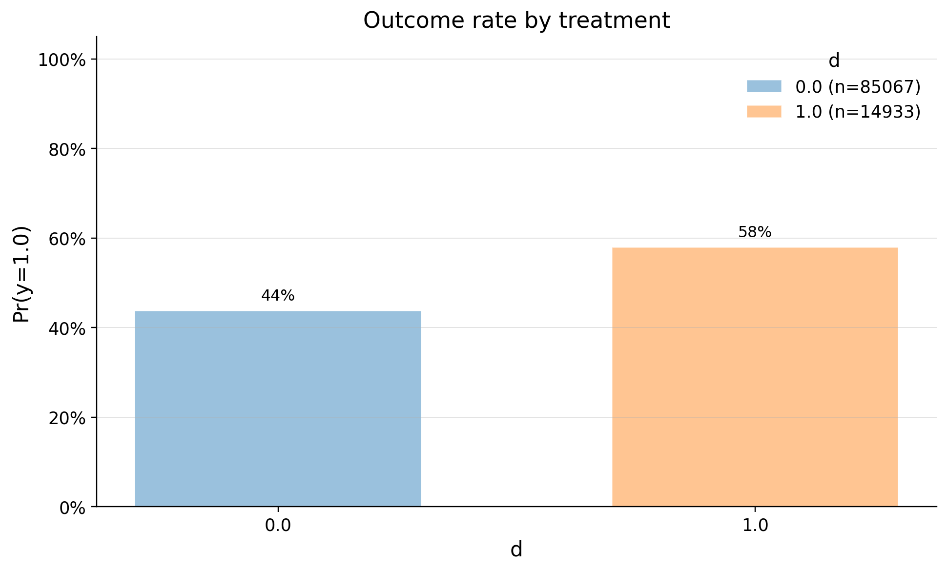
| treatment | count | mean | std | min | p10 | p25 | median | p75 | p90 | max | |
|---|---|---|---|---|---|---|---|---|---|---|---|
| 0 | 0.0 | 85067 | 0.437726 | 0.496110 | 0.0 | 0.0 | 0.0 | 0.0 | 1.0 | 1.0 | 1.0 |
| 1 | 1.0 | 14933 | 0.579388 | 0.493674 | 0.0 | 0.0 | 0.0 | 1.0 | 1.0 | 1.0 | 1.0 |
| confounders | mean_d_0 | mean_d_1 | abs_diff | smd | ks_pvalue | |
|---|---|---|---|---|---|---|
| 0 | spend_last_month | 83.486832 | 114.093736 | 30.606905 | 0.336140 | 0.00000 |
| 1 | premium_user | 0.237378 | 0.371325 | 0.133948 | 0.294234 | 0.00000 |
| 2 | avg_sessions_week | 4.823410 | 6.005089 | 1.181680 | 0.271347 | 0.00000 |
| 3 | prior_purchases_12m | 3.420633 | 3.802317 | 0.381684 | 0.190848 | 0.00000 |
| 4 | referred_user | 0.243197 | 0.310052 | 0.066855 | 0.149870 | 0.00000 |
| 5 | age_years | 36.594622 | 35.069304 | 1.525318 | -0.136350 | 0.00000 |
| 6 | email_opt_in | 0.542490 | 0.593652 | 0.051162 | 0.103421 | 0.00000 |
| 7 | mobile_user | 0.851270 | 0.882676 | 0.031406 | 0.092575 | 0.00000 |
| 8 | support_tickets_90d | 1.141982 | 1.243555 | 0.101572 | 0.091742 | 0.00000 |
| 9 | tenure_months | 28.338387 | 29.848652 | 1.510265 | 0.081531 | 0.00000 |
| 10 | weekend_user | 0.545370 | 0.575772 | 0.030402 | 0.061282 | 0.00000 |