generate_multitreatment_binary_26()
This notebook presents the generate multitreatment binary 26 research workflow and key analysis steps.
generate_multitreatment_binary_26() defines a 3-arm multi-treatment observational DGP with correlated confounders and a binary outcome.
Treatments are one-hot columns (d_0, d_1, d_2) and are sampled from a multinomial-logit propensity model calibrated toward target class shares .
1. Confounders and Copula Correlation
The confounder vector uses:
- (
tenure_months) , clipped to - (
weekly_active_days) , clipped to - (
annual_income_k) , clipped at 300 - (
premium_user) - (
family_plan) - (
recent_complaints) , clipped at 10 - (
discount_eligible) - (
engagement_score) with mean and concentration
Dependencies are induced with Gaussian copula correlation
2. Treatment Assignment (Softmax)
Class scores are with propensities
Scenario coefficients:
Treatment-score intercepts start at and are calibrated to match the target marginal rates.
3. Heterogeneous Effects on Logit Scale
Treatment shifts are additive on the link scale:
For d_1 (enforced harmful relative to control):
For d_2 (enforced beneficial relative to control):
4. Outcome Model (Binary Logistic)
Baseline logit: where
Observed logit under assigned treatment:
Then
5. Oracle Outputs
With include_oracle=True, the generated frame includes:
m_d_k: calibrated propensitiestau_link_d_k: link-scale treatment shiftsg_d_k: potential outcome probabilities under each armcate_d_1,cate_d_2: contrasts vs control on probability scale
| y | d_0 | d_1 | d_2 | tenure_months | weekly_active_days | annual_income_k | premium_user | family_plan | recent_complaints | ... | m_obs_d_1 | tau_link_d_1 | m_d_2 | m_obs_d_2 | tau_link_d_2 | g_d_0 | g_d_1 | g_d_2 | cate_d_1 | cate_d_2 | |
|---|---|---|---|---|---|---|---|---|---|---|---|---|---|---|---|---|---|---|---|---|---|
| 0 | 1.0 | 1.0 | 0.0 | 0.0 | 27.656605 | 2.649000 | 82.557046 | 0.0 | 1.0 | 0.0 | ... | 0.222533 | -0.410269 | 0.221226 | 0.221226 | 0.621091 | 0.462833 | 0.363730 | 0.615892 | -0.099103 | 0.153059 |
| 1 | 1.0 | 1.0 | 0.0 | 0.0 | 23.798386 | 2.771811 | 88.551369 | 0.0 | 0.0 | 2.0 | ... | 0.206692 | -0.467589 | 0.243357 | 0.243357 | 0.553028 | 0.467179 | 0.354558 | 0.603855 | -0.112621 | 0.136676 |
| 2 | 1.0 | 0.0 | 0.0 | 1.0 | 28.425009 | 2.793864 | 88.697176 | 0.0 | 0.0 | 0.0 | ... | 0.201852 | -0.420776 | 0.212748 | 0.212748 | 0.584368 | 0.551521 | 0.446713 | 0.688086 | -0.104807 | 0.136565 |
| 3 | 1.0 | 1.0 | 0.0 | 0.0 | 18.860066 | 3.303381 | 79.529890 | 0.0 | 0.0 | 1.0 | ... | 0.197248 | -0.454976 | 0.241111 | 0.241111 | 0.583534 | 0.523098 | 0.410350 | 0.662844 | -0.112748 | 0.139746 |
| 4 | 0.0 | 0.0 | 1.0 | 0.0 | 17.853087 | 2.605056 | 77.234837 | 0.0 | 0.0 | 0.0 | ... | 0.219363 | -0.410719 | 0.240004 | 0.240004 | 0.579375 | 0.581290 | 0.479350 | 0.712477 | -0.101940 | 0.131187 |
5 rows × 26 columns
Ground truth ATE for d_1 vs d_0 is -0.11659127048512116 Ground truth ATE for d_2 vs d_0 is 0.1380607452020492
MultiCausalData(df=(100000, 12), treatment_names=['d_0', 'd_1', 'd_2'], control_treatment='d_0')outcome='y', confounders=['tenure_months', 'weekly_active_days', 'annual_income_k', 'premium_user', 'family_plan', 'recent_complaints', 'discount_eligible', 'engagement_score'], user_id=None,
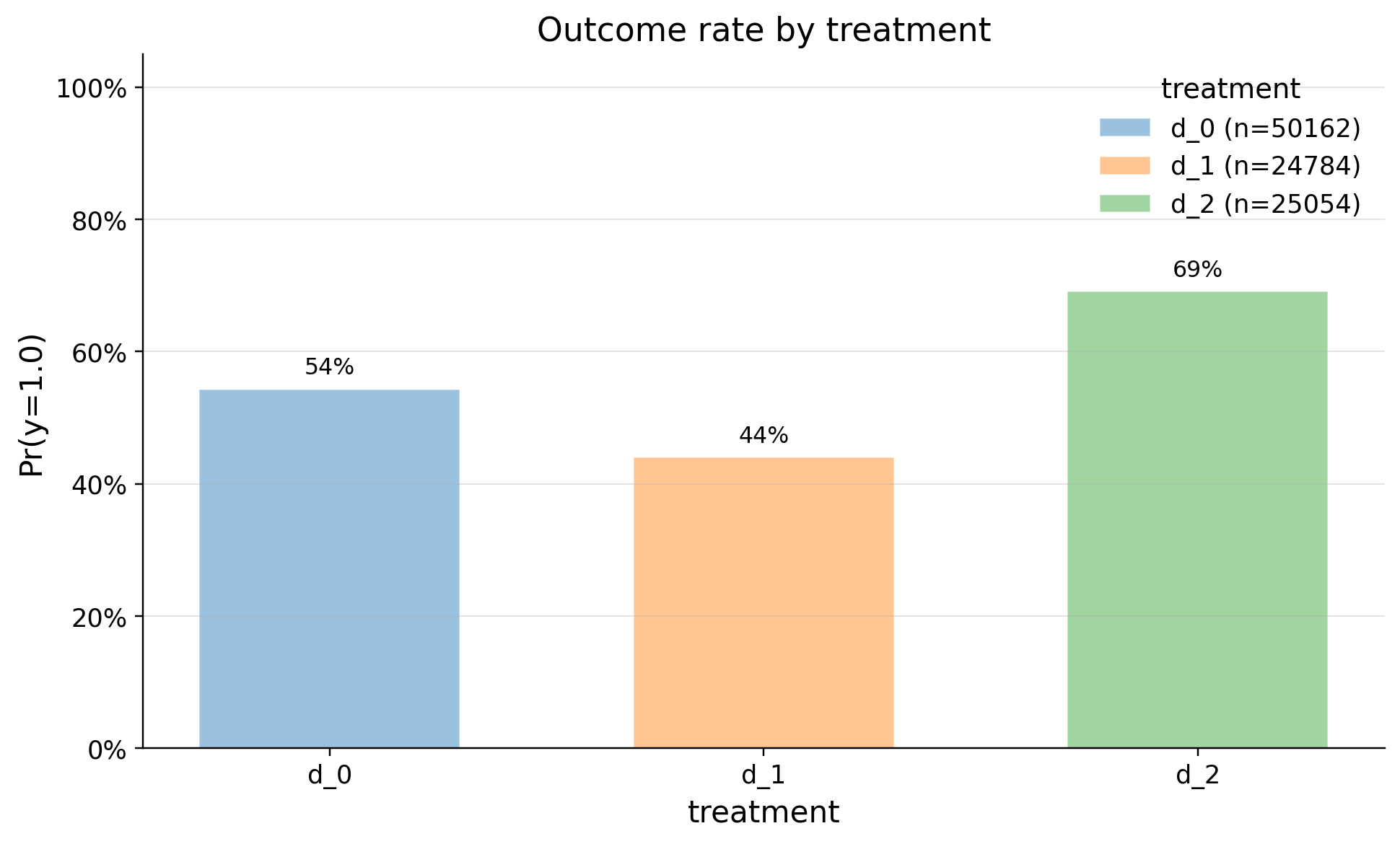
| treatment | count | mean | std | min | p10 | p25 | median | p75 | p90 | max | |
|---|---|---|---|---|---|---|---|---|---|---|---|
| 0 | d_0 | 50162 | 0.542881 | 0.498163 | 0.0 | 0.0 | 0.0 | 1.0 | 1.0 | 1.0 | 1.0 |
| 1 | d_2 | 25054 | 0.690389 | 0.462343 | 0.0 | 0.0 | 0.0 | 1.0 | 1.0 | 1.0 | 1.0 |
| 2 | d_1 | 24784 | 0.439517 | 0.496338 | 0.0 | 0.0 | 0.0 | 0.0 | 1.0 | 1.0 | 1.0 |
| confounders | mean_d_0 | mean_d_1 | abs_diff | smd | ks_pvalue | |
|---|---|---|---|---|---|---|
| 0 | premium_user | 0.189945 | 0.240880 | 0.050935 | 0.124134 | 0.00000 |
| 1 | weekly_active_days | 3.903170 | 4.013747 | 0.110577 | 0.075343 | 0.00000 |
| 2 | recent_complaints | 0.779395 | 0.845135 | 0.065740 | 0.072784 | 0.00000 |
| 3 | discount_eligible | 0.279116 | 0.305580 | 0.026464 | 0.058207 | 0.00000 |
| 4 | family_plan | 0.362924 | 0.390197 | 0.027273 | 0.056310 | 0.00000 |
| 5 | annual_income_k | 70.990667 | 72.151221 | 1.160554 | 0.032499 | 0.00069 |
| 6 | tenure_months | 23.747821 | 23.448586 | 0.299235 | -0.025648 | 0.00111 |
| 7 | engagement_score | 0.599728 | 0.602376 | 0.002649 | 0.022270 | 0.01979 |
| confounders | mean_d_0 | mean_d_1 | abs_diff | smd | ks_pvalue | |
|---|---|---|---|---|---|---|
| 0 | premium_user | 0.189945 | 0.263557 | 0.073613 | 0.176480 | 0.00000 |
| 1 | weekly_active_days | 3.903170 | 4.157551 | 0.254381 | 0.174018 | 0.00000 |
| 2 | tenure_months | 23.747821 | 25.549990 | 1.802169 | 0.153120 | 0.00000 |
| 3 | discount_eligible | 0.279116 | 0.335378 | 0.056262 | 0.122176 | 0.00000 |
| 4 | family_plan | 0.362924 | 0.412565 | 0.049640 | 0.102013 | 0.00000 |
| 5 | annual_income_k | 70.990667 | 73.516883 | 2.526216 | 0.070122 | 0.00000 |
| 6 | recent_complaints | 0.779395 | 0.805237 | 0.025842 | 0.028893 | 0.01295 |
| 7 | engagement_score | 0.599728 | 0.598192 | 0.001535 | -0.012894 | 0.29411 |