generate_cuped_tweedie_26
This notebook presents the generate cuped tweedie 26 research workflow and key analysis steps.
The generate_cuped_tweedie_26 data generating process (DGP) creates a synthetic dataset characterized by a Tweedie-like outcome (zero-inflated with a heavy right tail), correlated confounders, and structured heterogeneous treatment effects (HTE). It also includes pre-period covariates (y_pre and y_pre_2) calibrated for CUPED benchmarks.
1. Confounders
Five confounders are generated using a Gaussian Copula to induce specific correlations:
tenure_months():avg_sessions_week():spend_last_month():discount_rate():platform(): Categorical with levelsandroid(65%),ios(30%),web(5%).
Correlations: and .
2. Treatment Assignment
The treatment is assigned via a Bernoulli trial with a constant propensity score (RCT):
(Note: While the generator supports complex propensity models, generate_cuped_tweedie_26 defaults to a balanced random assignment).
3. Outcome Model
The outcome is generated as a two-part (hurdle) process:
A. Binary Indicator of Non-zero Outcome ()
- is the sigmoid function.
- (about 50% baseline non-zero rate).
- when
add_pre=True, and otherwise.
B. Positive Outcome Value ()
If , the value is drawn from a Gamma distribution:
- (shape parameter).
- , where is the log-mean linear predictor:
- .
- when
add_pre=True, and otherwise. - is a shared latent prognostic driver used in the outcome/pre construction (treatment remains randomized because ).
4. Heterogeneous Treatment Effect
The treatment effect is defined on the log-mean scale and incorporates monotone effects, diminishing returns, and categorical modifiers: Where:
- (saturating effect of tenure).
- (diminishing returns of sessions).
- (premium segment modifier).
generate_cuped_tweedie_26uses by default.
5. Pre-period Covariate
The first pre-period covariate uses the same latent driver that also drives outcome stochasticity when add_pre=True:
where is built from the Tweedie two-part mechanism, and is numerically calibrated so that \n
with default in generate_cuped_tweedie_26.
6. Second Pre-period Covariate
The second pre-period covariate is constructed from a second noisy view of the same latent driver (not an orthogonalized independent latent):
A. Latent-driven two-part base
With standardized covariates and :
B. Feasibility blending and calibration
If is below the second target, the base is blended with :
using the first on a grid that reaches the target (or the best achievable one). Then Gaussian noise is calibrated as:
to match the requested second control-group correlation. If pre_target_corr_2 is omitted, the default target is
| y | d | tenure_months | avg_sessions_week | spend_last_month | discount_rate | platform_ios | platform_web | m | m_obs | tau_link | g0 | g1 | cate | y_pre | _latent_A | y_pre_2 | |
|---|---|---|---|---|---|---|---|---|---|---|---|---|---|---|---|---|---|
| 0 | 3.734763 | 0.0 | 14.187461 | 2.0 | 57.355300 | 0.158164 | 1.0 | 0.0 | 0.5 | 0.5 | 0.103825 | 8.487966 | 9.416605 | 0.928639 | 17.972138 | 0.304717 | 10.783283 |
| 1 | 0.746406 | 1.0 | 6.352893 | 3.0 | 46.700946 | 0.085722 | 0.0 | 0.0 | 0.5 | 0.5 | 0.030781 | 8.487966 | 8.753301 | 0.265335 | 0.000000 | -1.039984 | 0.000000 |
| 2 | 13.040584 | 1.0 | 18.910153 | 9.0 | 80.136187 | 0.175115 | 1.0 | 0.0 | 0.5 | 0.5 | 0.357355 | 8.487966 | 12.133915 | 3.645949 | 34.771837 | 0.750451 | 24.866330 |
| 3 | 34.582113 | 1.0 | 7.927627 | 4.0 | 33.718224 | 0.152718 | 1.0 | 0.0 | 0.5 | 0.5 | 0.065554 | 8.487966 | 9.063025 | 0.575059 | 349.163943 | 0.940565 | 209.498366 |
| 4 | 0.000000 | 1.0 | 11.106925 | 2.0 | 92.064518 | 0.077390 | 0.0 | 0.0 | 0.5 | 0.5 | 0.056036 | 8.487966 | 8.977172 | 0.489206 | 0.000000 | -1.951035 | 0.243980 |
Ground truth ATE is 1.2383515933360814 Ground truth ATTE is 1.231529853520104
CausalData(df=(20000, 10), treatment='d', outcome='y', confounders=['tenure_months', 'avg_sessions_week', 'spend_last_month', 'discount_rate', 'platform_ios', 'platform_web', 'y_pre', 'y_pre_2'])
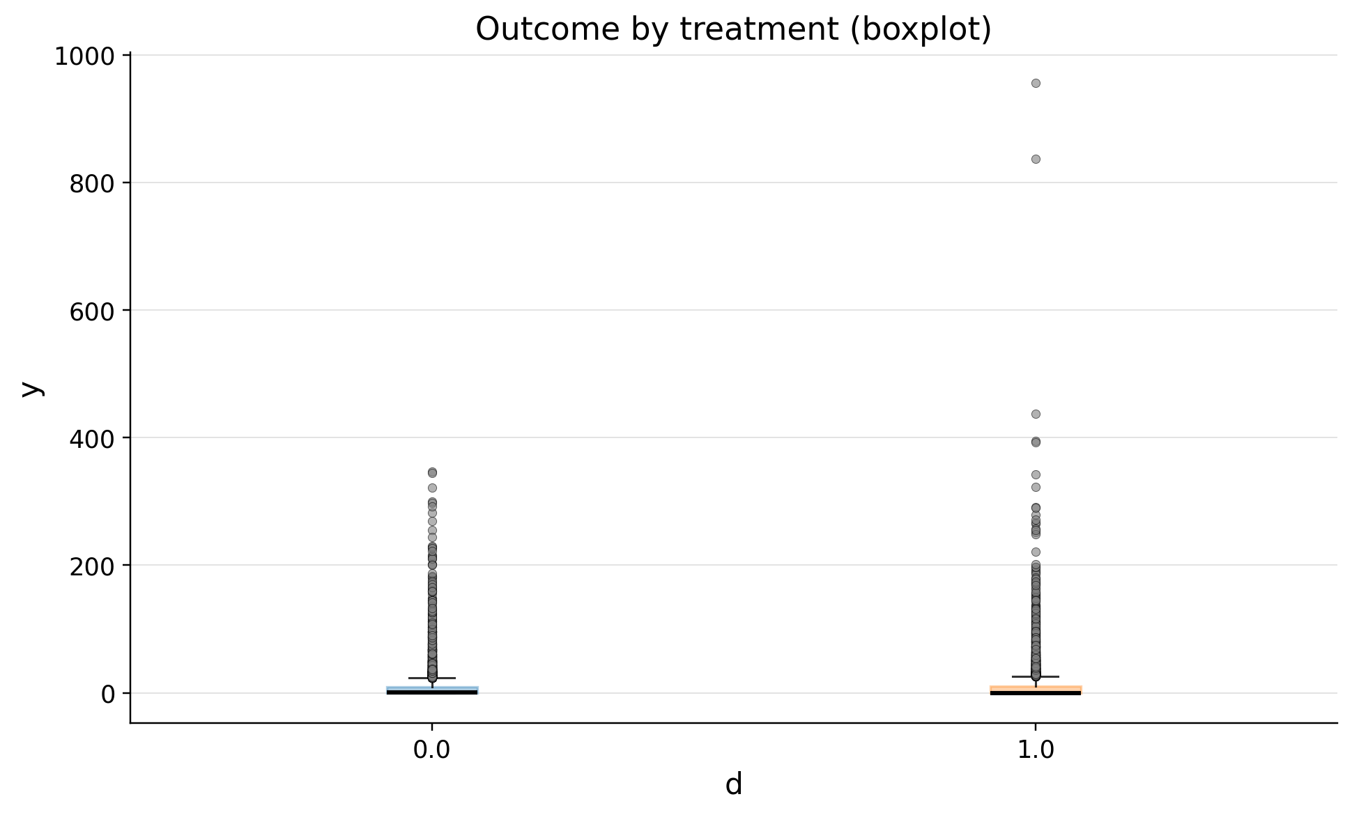
| treatment | count | mean | std | min | p10 | p25 | median | p75 | p90 | max | |
|---|---|---|---|---|---|---|---|---|---|---|---|
| 0 | 0.0 | 10049 | 8.867136 | 21.097599 | 0.0 | 0.0 | 0.0 | 0.276901 | 9.266134 | 24.454852 | 347.095992 |
| 1 | 1.0 | 9951 | 9.870188 | 25.879015 | 0.0 | 0.0 | 0.0 | 0.000000 | 10.409916 | 27.439125 | 956.413897 |
| confounders | mean_d_0 | mean_d_1 | abs_diff | smd | ks_pvalue | |
|---|---|---|---|---|---|---|
| 0 | tenure_months | 13.842686 | 13.615906 | 0.226781 | -0.030833 | 0.01991 |
| 1 | spend_last_month | 73.787667 | 75.159017 | 1.371350 | 0.019726 | 0.20812 |
| 2 | platform_ios | 0.304309 | 0.297357 | 0.006952 | -0.015158 | 0.96771 |
| 3 | y_pre | 7928.516448 | 20967.672427 | 13039.155979 | 0.014621 | 0.36084 |
| 4 | y_pre_2 | 4760.192129 | 12583.709202 | 7823.517073 | 0.014621 | 0.38473 |
| 5 | avg_sessions_week | 4.963379 | 5.015677 | 0.052297 | 0.012405 | 0.49401 |
| 6 | discount_rate | 0.100420 | 0.099996 | 0.000424 | -0.006421 | 0.36146 |
| 7 | platform_web | 0.050950 | 0.050749 | 0.000202 | -0.000918 | 1.00000 |