DGP generate_classic_rct_26
This notebook presents the generate classic rct 26 research workflow and key analysis steps.
Math Explanation of the generate_classic_rct_26 DGP
The generate_classic_rct_26 function generates a synthetic dataset for a Classic Randomized Controlled Trial (RCT). In this scenario, treatment is assigned completely at random, and covariates affect the outcome (prognostic) but do not influence the treatment assignment (no confounding).
By default, it simulates a conversion experiment (binary outcome) with 10,000 samples and a 50/50 split.
Covariate Generation (Confounders)
Three binary covariates are generated independently:
platform_ios():country_usa():source_paid():
Treatment Assignment ()
Since it is an RCT, the treatment is independent of . It is assigned with a probability : The log-odds of treatment (intercept ) is .
Outcome Generation (conversion)
The outcome is a binary variable representing conversion. The probability of conversion for an individual is modeled using a logistic link function: where is the sigmoid function.
The latent linear predictor is defined as:
By default, because add_pre=False. The nonlinear term is only included when add_pre=True (or when g_y/use_prognostic is provided).
- Baseline Intercept (): Derived from the target control conversion rate . This sets the baseline rate at ; the marginal control rate can differ once shifts log-odds.
- Treatment Effect (): Derived from the target treatment conversion rate . It represents the shift in log-odds. This is a baseline log-odds shift; the marginal ATE on the probability scale is not exactly 1% once effects are present.
- Prognostic Coefficients (): By default, . These values determine how much each covariate shifts the log-odds of conversion.
The outcome is a binary variable representing conversion. The probability of conversion for an individual is modeled using a logistic link function: where is the sigmoid function.
The latent linear predictor is defined as:
- Baseline Intercept (): Derived from the target control conversion rate .
- Treatment Effect (): Derived from the target treatment conversion rate . It represents the shift in log-odds. On the probability scale, this corresponds to an Average Treatment Effect (ATE) of .
- Prognostic Coefficients (): By default, . These values determine how much each covariate shifts the log-odds of conversion.
Summary of Default Parameters
- : 10,000
- Control Conversion (baseline ): 10% at (marginal rate can differ with )
- Treatment Conversion (baseline ): 11% at (marginal rate can differ with )
- Treatment Split: 50%
- Confounders: 3 binary
- Nonlinear : only when
add_pre=Trueorg_y/use_prognosticis provided
DGP
| user_id | conversion | d | platform_ios | country_usa | source_paid | m | m_obs | tau_link | g0 | g1 | cate | |
|---|---|---|---|---|---|---|---|---|---|---|---|---|
| 0 | 8826d | 0.0 | 0.0 | 1.0 | 0.0 | 1.0 | 0.5 | 0.5 | 0.106483 | 0.310620 | 0.333868 | 0.023249 |
| 1 | 2416d | 0.0 | 1.0 | 0.0 | 0.0 | 1.0 | 0.5 | 0.5 | 0.106483 | 0.198257 | 0.215727 | 0.017471 |
| 2 | eb819 | 0.0 | 0.0 | 1.0 | 1.0 | 0.0 | 0.5 | 0.5 | 0.106483 | 0.231969 | 0.251479 | 0.019509 |
| 3 | 71445 | 0.0 | 1.0 | 1.0 | 1.0 | 0.0 | 0.5 | 0.5 | 0.106483 | 0.231969 | 0.251479 | 0.019509 |
| 4 | 13d16 | 0.0 | 1.0 | 0.0 | 1.0 | 0.0 | 0.5 | 0.5 | 0.106483 | 0.142189 | 0.155678 | 0.013489 |
Ground truth ATE is 0.01719144406311028 Ground truth ATTE is 0.017278385179220486
CausalData(df=(10000, 5), treatment='d', outcome='conversion', confounders=['platform_ios', 'country_usa', 'source_paid'])
EDA
| treatment | count | mean | std | min | p10 | p25 | median | p75 | p90 | max | |
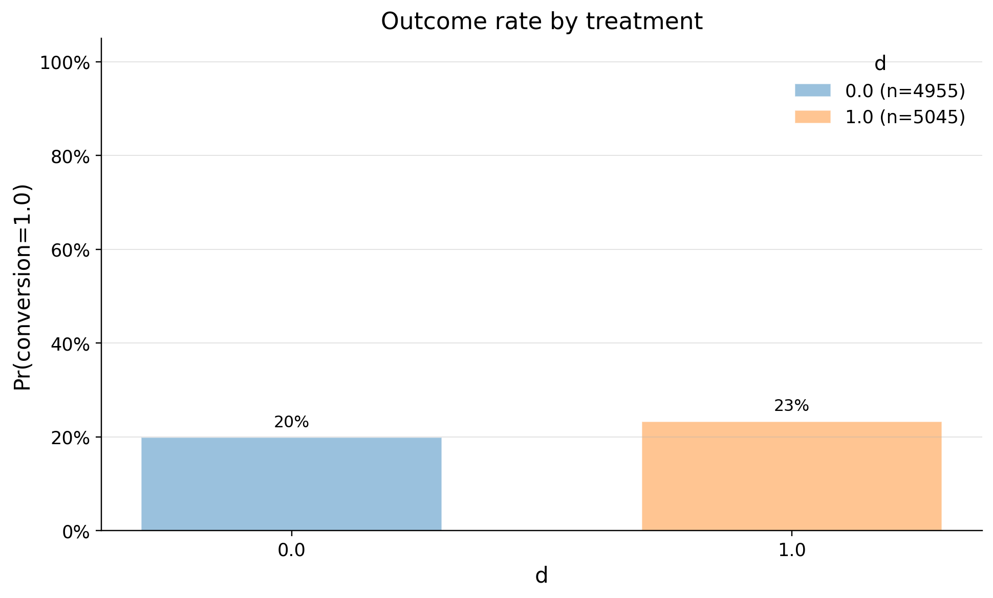
|---|---|---|---|---|---|---|---|---|---|---|---|
| 0 | 0.0 | 4955 | 0.198991 | 0.399281 | 0.0 | 0.0 | 0.0 | 0.0 | 0.0 | 1.0 | 1.0 |
| 1 | 1.0 | 5045 | 0.232904 | 0.422723 | 0.0 | 0.0 | 0.0 | 0.0 | 0.0 | 1.0 | 1.0 |
Balance check
| confounders | mean_d_0 | mean_d_1 | abs_diff | smd | ks_pvalue | |
|---|---|---|---|---|---|---|
| 0 | source_paid | 0.299092 | 0.313776 | 0.014684 | 0.031853 | 0.64592 |
| 1 | platform_ios | 0.494046 | 0.502874 | 0.008828 | 0.017654 | 0.98861 |
| 2 | country_usa | 0.586276 | 0.591873 | 0.005597 | 0.011374 | 1.00000 |