GATE

We call 'GATE' a scenario where in observational study after fitting DML model we analyzing treatment effect heterogeneity between groups of clients

Data

We will use DGP from Causalis. Read more at https://causalis.causalcraft.com/articles/generate_obs_hte_26_rich

Result

	user_id	y	d	tenure_months	avg_sessions_week	spend_last_month	age_years	income_monthly	prior_purchases_12m	support_tickets_90d	premium_user	mobile_user	urban_resident	referred_user	m	m_obs	tau_link	g0	g1	cate
0	1	0.000000	0.0	28.814654	1.0	77.936767	50.234101	1926.698301	1.0	2.0	1.0	1.0	1.0	0.0	0.045453	0.045453	0.089095	8.137981	9.142395	1.004414
1	2	80.099611	1.0	25.913345	3.0	53.777740	28.115859	5104.271509	3.0	0.0	1.0	1.0	0.0	1.0	0.041514	0.041514	0.246679	60.459257	78.817307	18.358049
2	3	6.400482	1.0	24.969929	10.0	134.764322	22.907062	5267.938255	8.0	3.0	0.0	1.0	1.0	0.0	0.052593	0.052593	0.162968	7.712855	9.138577	1.425723
3	4	2.788238	0.0	40.655089	5.0	59.517074	31.970490	6597.327018	3.0	2.0	1.0	1.0	1.0	0.0	0.036221	0.036221	0.188755	25.386510	31.159932	5.773422
4	5	0.000000	0.0	18.560899	3.0	74.370930	39.237248	4930.009628	5.0	1.0	1.0	1.0	0.0	0.0	0.036343	0.036343	0.174757	15.359250	18.600227	3.240977

Result

Ground truth ATE is 19.409586529660793 Ground truth ATTE is 10.914991423363865

Result

CausalData(df=(100000, 14), treatment='d', outcome='y', confounders=['tenure_months', 'avg_sessions_week', 'spend_last_month', 'age_years', 'income_monthly', 'prior_purchases_12m', 'support_tickets_90d', 'premium_user', 'mobile_user', 'urban_resident', 'referred_user'], user_id='user_id')

Result

	treatment	count	mean	std	min	p10	p25	median	p75	p90	max
0	0.0	95051	76.087138	240.800713	0.0	0.0	0.0	8.39544	64.859278	190.227900	21396.007575
1	1.0	4949	58.506172	199.485625	0.0	0.0	0.0	0.00000	36.958280	148.837193	5143.642132

Our data has strong treatment class disbalance. Only 5% of sample activated in treatment.

Treatment group has lower mean LTV. It's too early to draw conclusions.

Result

png

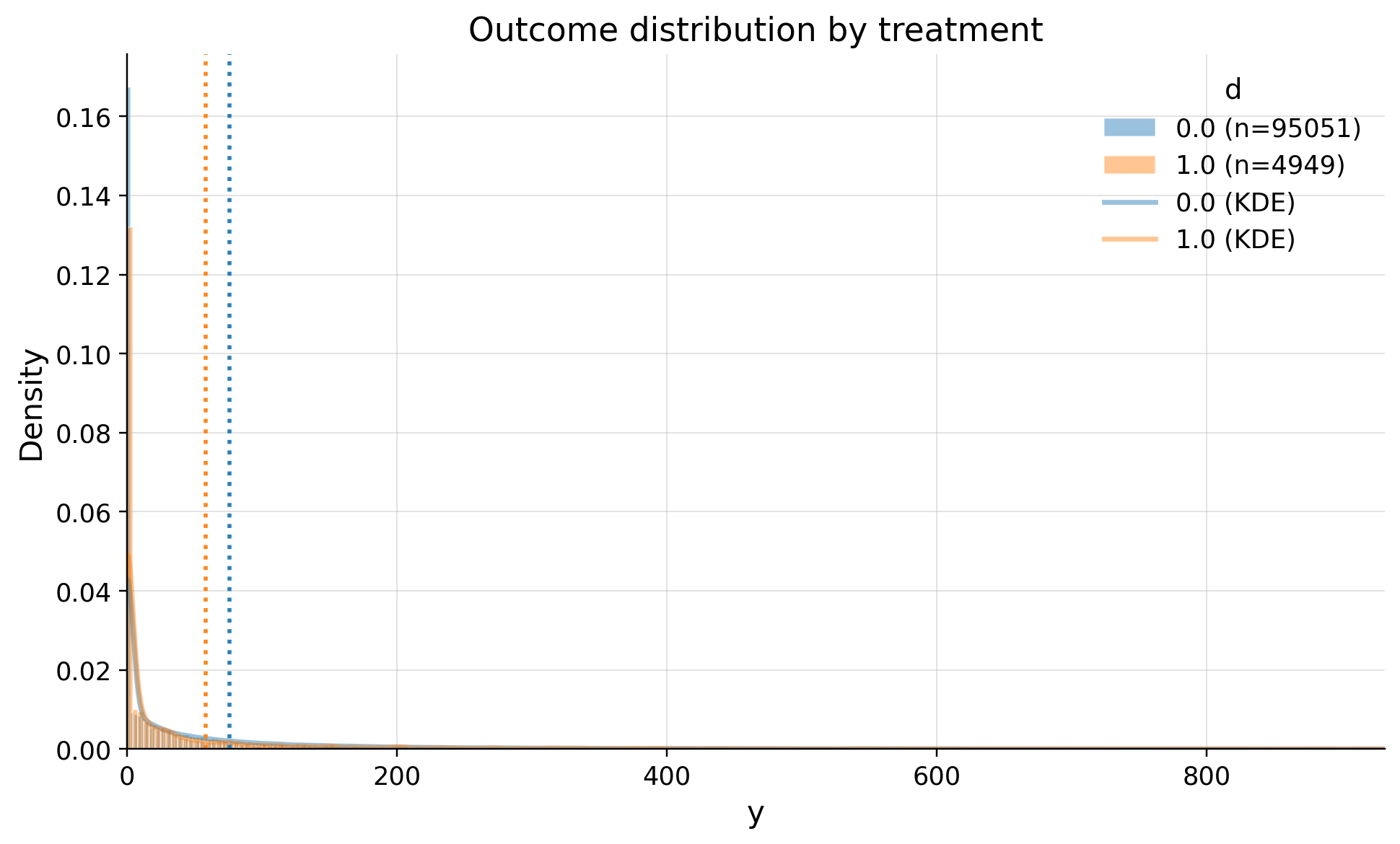
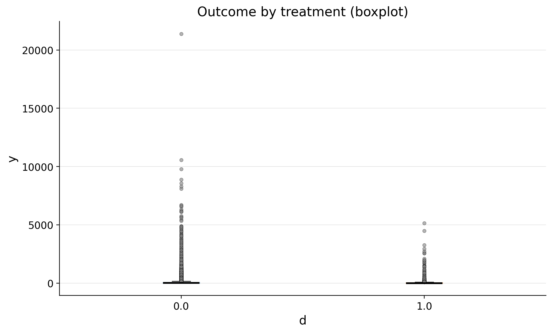
We see large right tale

Result

png

Result

	treatment	n	outlier_count	outlier_rate	lower_bound	upper_bound	has_outliers	method	tail
0	0.0	95051	11300	0.118884	-97.288916	162.148194	True	iqr	both
1	1.0	4949	721	0.145686	-55.437420	92.395699	True	iqr	both

We see many outliers. It's common situation for LTV metric. Dropping them will lead to a biased conclusion

Result

	confounders	mean_d_0	mean_d_1	abs_diff	smd	ks_pvalue
0	premium_user	0.751807	0.591837	0.159970	-0.345721	0.00000
1	income_monthly	4549.385190	3918.058798	631.326392	-0.277611	0.00000
2	spend_last_month	89.091801	67.375389	21.716412	-0.268360	0.00000
3	support_tickets_90d	0.984545	1.259244	0.274699	0.253974	0.00000
4	avg_sessions_week	5.047753	4.230148	0.817606	-0.201735	0.00000
5	prior_purchases_12m	3.904220	3.513639	0.390581	-0.189372	0.00000
6	tenure_months	28.740100	25.559161	3.180939	-0.184156	0.00000
7	age_years	36.435984	34.809083	1.626901	-0.144142	0.00000
8	referred_user	0.271486	0.307133	0.035647	0.078671	0.00001
9	urban_resident	0.600793	0.568802	0.031991	-0.064954	0.00013
10	mobile_user	0.874573	0.870075	0.004498	-0.013477	0.99998

As we see clients are differ on this confounders. We need to controll them to make causal inference

ATTE

ATTE is right estimand here. We will estimate effect on clients that were treated, had first purchase in our product

Result

	value
field
estimand	ATTE
model	IRM
value	11.7030 (ci_abs: 7.2449, 16.1611)
value_relative	25.0048 (ci_rel: 15.3806, 34.6290)
alpha	0.0500
p_value	0.0000
is_significant	True
n_treated	4949
n_control	95051
treatment_mean	58.5062
control_mean	76.0871
time	2026-04-09

Our estimate is 12.1542 dollars (ci_abs: 7.7933, 16.5152). Mean in treatment group is 58.5062 dollars, so without our product it would be 46.3520 dollars.

GATET

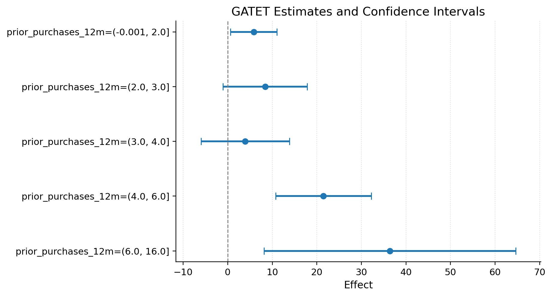
Quantile groups GATET

Result

	group	value	is_significant	ci_lower	ci_upper	n_group	n_treated	n_control	share_treated	std_error	test_stat	p_value	mean_phi	std_phi	mean_propensity	min_propensity	max_propensity
0	prior_purchases_12m=(-0.001, 2.0]	5.815230	True	0.588179	11.042281	27484	1700	25784	0.06185	2.666912	2.180511	0.02922	5.815230	442.653459	0.059719	0.01	0.823073
1	prior_purchases_12m=(2.0, 3.0]	8.376332	False	-1.083934	17.836598	19182	984	18198	0.05130	4.826755	1.735396	0.08267	8.376332	670.049474	0.050492	0.01	0.583411
2	prior_purchases_12m=(3.0, 4.0]	3.922010	False	-5.991967	13.835987	18236	847	17389	0.04645	5.058245	0.775370	0.43812	3.922010	683.288078	0.045796	0.01	0.519778
3	prior_purchases_12m=(4.0, 6.0]	21.469848	True	10.726077	32.213618	23812	1014	22798	0.04258	5.481616	3.916700	0.00009	21.469848	851.744757	0.041627	0.01	0.463650
4	prior_purchases_12m=(6.0, 16.0]	36.380628	True	8.129337	64.631919	11286	404	10882	0.03580	14.414189	2.523946	0.01160	36.380628	1543.213691	0.033757	0.01	0.554571

Result

png

Integer groups GATET

Result

	group	value	is_significant	ci_lower	ci_upper	n_group	n_treated	n_control	share_treated	std_error	test_stat	p_value	mean_phi	std_phi	mean_propensity	min_propensity	max_propensity
0	mobile_user=0.0	5.740115	False	-0.723297	12.203527	12565	643	11922	0.05117	3.297720	1.740632	0.08175	5.740115	370.360716	0.048592	0.01	0.823073
1	mobile_user=1.0	12.593462	True	7.562008	17.624917	87435	4306	83129	0.04925	2.567116	4.905686	0.00000	12.593462	761.259047	0.048112	0.01	0.617166

Formal group comparisons

result.summary() answers which subgroup effects are different from 0.
result.contrast(...) answers whether one subgroup effect differs from another.
result.pairwise_summary(reference=...) compares every subgroup against a chosen reference group.

Result

	value
field
estimand	GATET_CONTRAST
model	IRM
contrast	mobile_user=1.0 - mobile_user=0.0
left_group	mobile_user=1.0
right_group	mobile_user=0.0
value	6.8533 (ci_abs: -1.3376, 15.0443)
std_error	4.1791
test_stat	1.6399
alpha	0.0500
alternative	two-sided
p_value	0.1010
is_significant	False
left_value	12.5935
right_value	5.7401
n_left	87435
n_right	12565
time	2026-04-09

Result

	left_group	right_group	contrast_label	left_value	right_value	estimate_diff	std_error	test_stat	p_value	p_value_adj	ci_lower	ci_upper	is_significant	is_significant_adj	n_left	n_right	alpha	p_adjust
0	mobile_user=1.0	mobile_user=0.0	mobile_user=1.0 - mobile_user=0.0	12.593462	5.740115	6.853347	4.179119	1.639902	0.101025	0.101025	-1.337576	15.044271	False	False	87435	12565	0.05	none

Manual groups GATET

Result

	group	value	is_significant	ci_lower	ci_upper	n_group	n_treated	n_control	share_treated	std_error	test_stat	p_value	mean_phi	std_phi	mean_propensity	min_propensity	max_propensity
0	0=Middle	9.255211	True	2.743687	15.766736	57050	2633	54417	0.04615	3.322268	2.785812	0.00534	9.255211	794.703618	0.045350	0.01	0.823073
1	0=Senior	7.901003	False	-9.123459	24.925465	12133	504	11629	0.04154	8.686110	0.909614	0.36303	7.901003	958.003435	0.039543	0.01	0.601238
2	0=Young	16.317476	True	10.295807	22.339144	30817	1812	29005	0.05880	3.072336	5.311097	0.00000	16.317476	543.248095	0.056793	0.01	0.617166

Multi-column indicator groups GATET

Yes. groups= for score="GATET" can be a multi-column DataFrame of 0/1 subgroup indicators.

The columns must define a strict partition of the fitted sample:

every column must be binary,
every row must belong to exactly one subgroup,
every subgroup must contain at least one treated observation.

Groups with no controls are still accepted for GATET, but the estimator emits a warning because within-group overlap is degenerate.

Result

	group	value	is_significant	ci_lower	ci_upper	n_group	n_treated	n_control	share_treated	std_error	test_stat	p_value	mean_phi	std_phi	mean_propensity	min_propensity	max_propensity
0	Middle_mobile=0	4.351636	False	-4.224174	12.927446	7511	362	7149	0.04820	4.375494	0.994547	0.31996	4.351636	379.777268	0.046450	0.01	0.823073
1	Middle_mobile=1	10.036847	True	2.612594	17.461100	49539	2271	47268	0.04584	3.787954	2.649675	0.00806	10.036847	844.395048	0.045183	0.01	0.604030
2	Senior_mobile=0	5.735265	False	-15.356013	26.826542	2500	113	2387	0.04520	10.761053	0.532965	0.59406	5.735265	537.725806	0.041483	0.01	0.439237
3	Senior_mobile=1	8.526907	False	-12.552376	29.606190	9633	391	9242	0.04059	10.754934	0.792837	0.42787	8.526907	1057.209477	0.039040	0.01	0.601238
4	Young_mobile=0	8.735219	True	0.417677	17.052762	2554	168	2386	0.06578	4.243722	2.058386	0.03955	8.735219	217.072946	0.061850	0.01	0.386215
5	Young_mobile=1	17.092305	True	10.510944	23.673665	28263	1644	26619	0.05817	3.357899	5.090179	0.00000	17.092305	568.645110	0.056336	0.01	0.617166