DML ATE Example

This notebook covers scenario: | Is RCT | Treatment | Outcome | EDA | Estimands | Refutation | |---------------|-----------|------------|-----|-----------|------------| | Observational | Binary | Continuous | Yes | ATE | Yes |

We will estimate Average Treatment Effect (ATE) of binary treatment on continuous outcome. It shows explonatary data analysis and refutation tests

Generate data

Let's generate data of how feature (Treatment) impact on ARPU (Outcome) with linear effect (theta) = 1.8

Result

	y	d	tenure_months	avg_sessions_week	spend_last_month	premium_user	urban_resident
0	4.127714	0.0	27.656605	5.352554	72.552568	1.0	0.0
1	11.122008	1.0	11.520191	6.798247	188.481287	1.0	0.0
2	10.580393	1.0	33.005414	2.055459	51.040440	0.0	1.0
3	6.982844	1.0	35.286777	4.429404	166.992239	0.0	1.0
4	10.899381	0.0	0.587578	6.658307	179.371126	0.0	0.0

EDA

Result

{'n_rows': 10000, 'n_columns': 7}

General dataset information

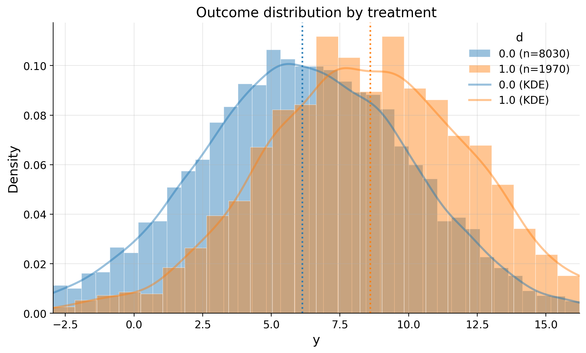
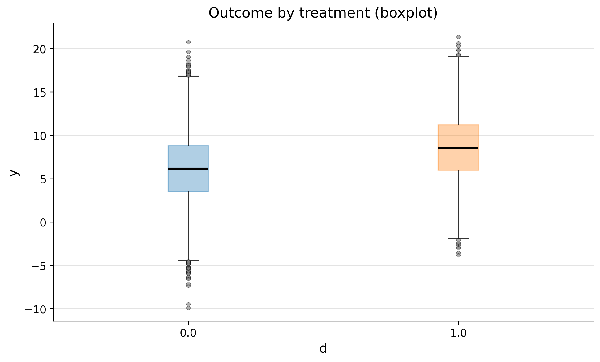
Let's see how outcome differ between clients who recieved the feature and didn't

Result

	count	mean	std	min	p10	p25	median	p75	p90	max
treatment
0.0	8030	6.137433	3.933863	-9.866447	1.118291	3.517427	6.157583	8.847907	11.114776	20.770359
1.0	1970	8.608973	3.942856	-3.821492	3.666892	5.986613	8.560912	11.247429	13.552612	21.377687

Result

png

Result

png

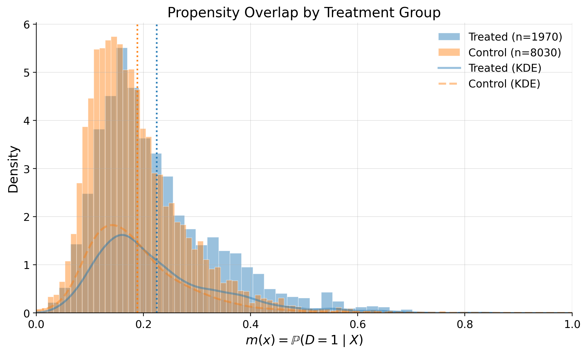
Propensity

Now let's examine how propensity score differ treatments

Result

	mean_t_0	mean_t_1	abs_diff	smd	ks	ks_pvalue
confounders
premium_user	0.218057	0.382234	0.164176	0.364037	0.164176	1.061599e-37
tenure_months	23.405355	25.799499	2.394143	0.199024	0.087485	5.511096e-11
avg_sessions_week	4.976354	5.302999	0.326645	0.163509	0.075782	2.382131e-08
urban_resident	0.587547	0.655330	0.067783	0.140072	0.067783	9.127269e-07
spend_last_month	99.288113	104.941250	5.653137	0.097172	0.057348	5.761025e-05

Result

ROC AUC from PropensityModel: 0.5926

Result

Positivity check from PropensityModel: {'bounds': (0.05, 0.95), 'share_below': 0.0121, 'share_above': 0.0, 'flag': False}

Result

	feature	shap_mean	shap_mean_abs	exact_pp_change_abs	exact_pp_change_signed
0	num__spend_last_month	0.000299	0.166002	0.027438	0.000047
1	num__premium_user	-0.000269	0.306301	0.052687	-0.000042
2	num__urban_resident	0.000245	0.158900	0.026210	0.000039
3	num__avg_sessions_week	-0.000141	0.174082	0.028841	-0.000022
4	num__tenure_months	-0.000135	0.194878	0.032482	-0.000021

Result

png

Outcome regression

Let's analyze how confounders predict outcome

Result

{'rmse': 3.656989617205263, 'mae': 2.90424413216463}

Result

	feature	shap_mean
0	avg_sessions_week	-0.000502
1	spend_last_month	0.000350
2	urban_resident	0.000245
3	premium_user	-0.000055
4	tenure_months	-0.000038

Inference

Now time to estimate ATE with Double Machine Learning

Result

1.766253520771568 0.0 (1.5329683790491713, 1.9995386624939646)

True theta in our data generating proccess was 1.8

Refutation

Overlap

Result

	metric	value	flag
0	edge_0.01_below	0.000000	GREEN
1	edge_0.01_above	0.000000	GREEN
2	edge_0.02_below	0.001000	GREEN
3	edge_0.02_above	0.000000	GREEN
4	KS	0.139672	GREEN
5	AUC	0.592382	GREEN
6	ESS_treated_ratio	0.742224	GREEN
7	ESS_control_ratio	0.970455	GREEN
8	tails_w1_q99/med	6.278831	GREEN
9	tails_w0_q99/med	2.844508	GREEN
10	ATT_identity_relerr	0.037683	GREEN
11	clip_m_total	0.000100	GREEN
12	calib_ECE	0.036215	GREEN
13	calib_slope	0.520588	RED
14	calib_intercept	-0.637457	RED

Score

Result

	metric	value	flag
0	se_plugin	1.190252e-01	NA
1	psi_p99_over_med	1.355647e+01	YELLOW
2	psi_kurtosis	6.047594e+01	RED
3	max_\|t\|_g1	5.463687e+00	RED
4	max_\|t\|_g0	1.384511e+00	GREEN
5	max_\|t\|_m	1.388284e+00	GREEN
6	oos_tstat_fold	1.241609e-15	GREEN
7	oos_tstat_strict	1.241615e-15	GREEN

SUTVA

Result

1.) Are your clients independent (i)? 2.) Do you measure confounders, treatment, and outcome in the same intervals? 3.) Do you measure confounders before treatment and outcome after? 4.) Do you have a consistent label of treatment, such as if a person does not receive a treatment, he has a label 0?

Uncofoundedness

Result

	metric	value	flag
0	balance_max_smd	0.021956	GREEN
1	balance_frac_violations	0.000000	GREEN

Result

{'theta': 1.766253520771568, 'se': 0.11902521860734187, 'level': 0.95, 'z': 1.959963984540054, 'sampling_ci': (1.5329683790491713, 1.9995386624939646), 'theta_bounds_confounding': (1.6875916811818483, 1.8449153603612876), 'bias_aware_ci': (1.4543065394594517, 2.0782005020836842), 'max_bias': 0.07866183958971962, 'sigma2': 13.136641553423134, 'nu2': 0.43676740621591587, 'params': {'cf_y': 0.01, 'cf_d': 0.01, 'rho': 1.0, 'use_signed_rr': False}}

Result

	cf_y	cf_d	rho	theta_long	theta_short	delta
d	0.000034	3.037675e-07	-1.0	1.766254	1.845679	-0.079425