DGP classic_rct_gamma_26
This notebook presents the classic rct gamma 26 research workflow and key analysis steps.
Math Explanation of the classic_rct_gamma_26 DGP
The classic_rct_gamma_26 function generates a synthetic dataset for a Classic Randomized Controlled Trial (RCT). Treatment is assigned completely at random, and covariates affect the outcome (prognostic) but do not influence treatment assignment (no confounding).
By default, it simulates a revenue experiment (gamma outcome) with 10,000 samples and a 50/50 split.
Covariate Generation (Confounders)
Three binary covariates are generated independently:
platform_ios():country_usa():source_paid():
Treatment Assignment ()
Since it is an RCT, the treatment is independent of . It is assigned with a probability : The log-odds of treatment (intercept ) is .
Outcome Generation (revenue)
The outcome is a positive, skewed metric (e.g., revenue) modeled with a Gamma distribution using a log-mean link:
By default, because add_pre=False. The nonlinear term is only included when add_pre=True (or when g_y/use_prognostic is provided).
- Shape (): Default .
- Scale (control ): Default .
- Scale (treatment ): Default .
- Prognostic Coefficients (): Default . These values shift the log-mean of revenue.
With the defaults, the group means are: This corresponds to a 10% uplift on the mean scale before covariate effects.
Summary of Default Parameters
- : 10,000
- Control Mean (baseline): at
- Treatment Mean (baseline): at
- Treatment Split: 50%
- Confounders: 3 binary
- Nonlinear : only when
add_pre=Trueorg_y/use_prognosticis provided
DGP
| user_id | revenue | d | platform_ios | country_usa | source_paid | age | cnt_trans | platform_Android | platform_iOS | invited_friend | m | m_obs | tau_link | g0 | g1 | cate | |
|---|---|---|---|---|---|---|---|---|---|---|---|---|---|---|---|---|---|
| 0 | ae006 | 62.015001 | 0.0 | 1.0 | 0.0 | 1.0 | 39 | 0 | 0 | 1 | 0 | 0.5 | 0.5 | 0.09531 | 60.412581 | 66.453839 | 6.041258 |
| 1 | 6051e | 22.353186 | 1.0 | 0.0 | 0.0 | 1.0 | 46 | 4 | 0 | 1 | 0 | 0.5 | 0.5 | 0.09531 | 47.049366 | 51.754302 | 4.704937 |
| 2 | eb08c | 38.213100 | 0.0 | 1.0 | 1.0 | 0.0 | 36 | 1 | 1 | 0 | 0 | 0.5 | 0.5 | 0.09531 | 47.049366 | 51.754302 | 4.704937 |
| 3 | a947a | 77.927095 | 1.0 | 1.0 | 1.0 | 0.0 | 26 | 2 | 0 | 1 | 0 | 0.5 | 0.5 | 0.09531 | 47.049366 | 51.754302 | 4.704937 |
| 4 | 9bd42 | 24.936085 | 1.0 | 0.0 | 1.0 | 0.0 | 35 | 3 | 0 | 1 | 0 | 0.5 | 0.5 | 0.09531 | 36.642083 | 40.306291 | 3.664208 |
Ground truth ATE is 4.547002938251698 Ground truth ATTE is 4.571328700457634
CausalData(df=(10000, 5), treatment='d', outcome='revenue', confounders=['platform_ios', 'country_usa', 'source_paid'])
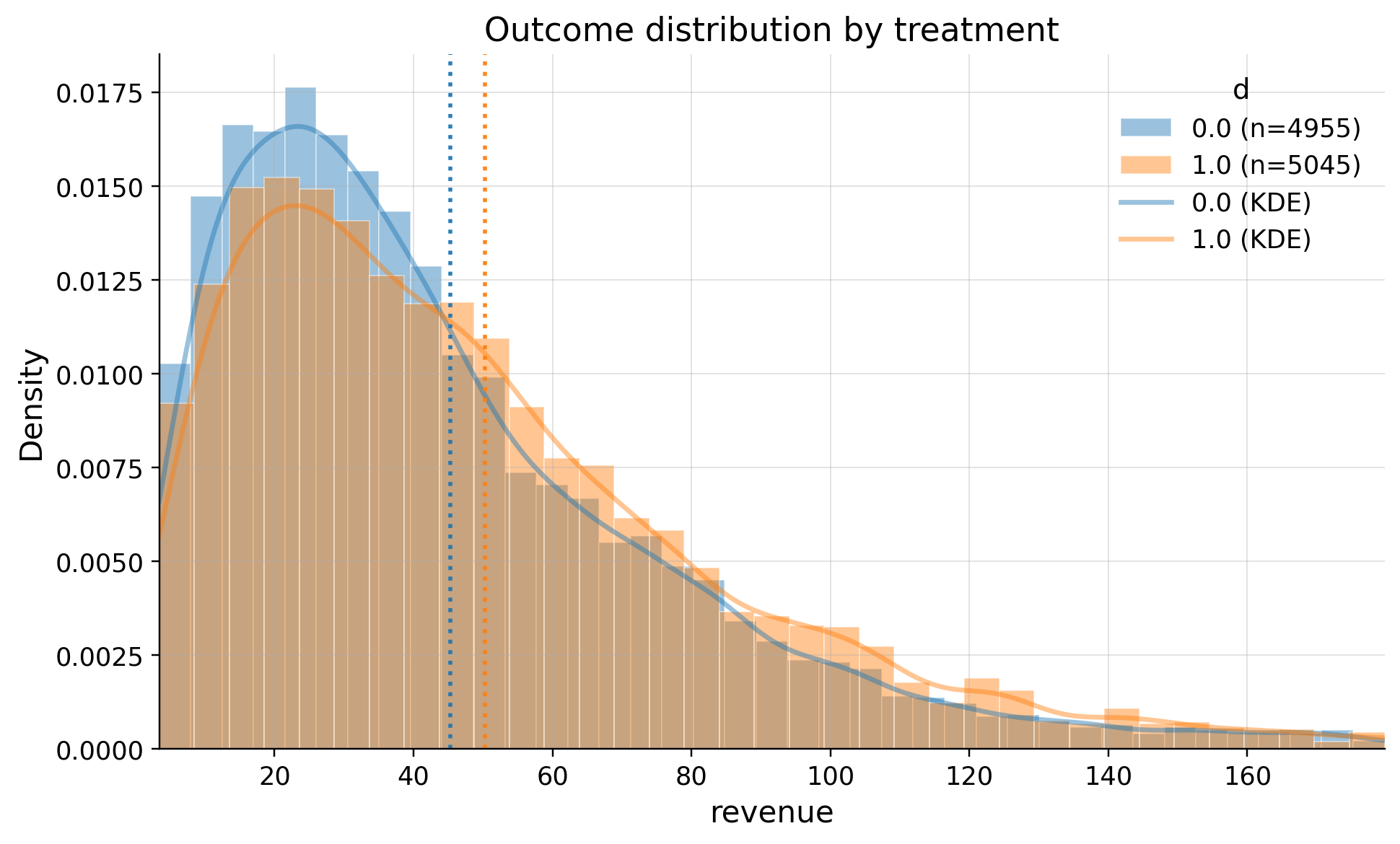
EDA
| treatment | count | mean | std | min | p10 | p25 | median | p75 | p90 | max | |
|---|---|---|---|---|---|---|---|---|---|---|---|
| 0 | 0.0 | 4955 | 45.271228 | 36.185063 | 0.338380 | 11.081530 | 20.326602 | 35.784254 | 60.063958 | 89.576241 | 431.357219 |
| 1 | 1.0 | 5045 | 50.328883 | 38.802710 | 0.448255 | 12.335521 | 22.792900 | 41.149396 | 67.409299 | 100.121519 | 401.883422 |
Balance check
| confounders | mean_d_0 | mean_d_1 | abs_diff | smd | ks_pvalue | |
|---|---|---|---|---|---|---|
| 0 | source_paid | 0.299092 | 0.313776 | 0.014684 | 0.031853 | 0.64592 |
| 1 | platform_ios | 0.494046 | 0.502874 | 0.008828 | 0.017654 | 0.98861 |
| 2 | country_usa | 0.586276 | 0.591873 | 0.005597 | 0.011374 | 1.00000 |